Procedural generation

Procedural generation involves generating a world through mathematics instead of manually hand-crafting it. The world is randomly generated but deterministic from its seed. This allows for both infinite worlds, with huge variance in their appearance and gameplay experience, and reduced cost of development and maintenance of assets and maps through carefully generated noise and randomness providing worlds comparable in quality to hand-crafted ones. This also allows the base chunks to never be stored as they can always be retrieved, saving work for both artists and the computer.

This article explores how some techniques function, and introduces implementation details of techniques and tools such as SDFs, noise, splines and some analytic techniques. It also introduces concepts such as constraints and local control, and their use in fine-tuning and modelling approaches more appropriate for given tasks.

From random values to smooth noise

The most trivial random number generation technique would be to come up with a random float between 0 and 1 for each cell and scale it.

$f(x) \to \operatorname{random}(0,1)$

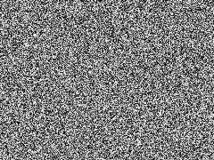
This might work for certain cases, and is certainly involved in all others as a foundation to be built upon. But for most cases this approach offers little spatial control and has no continuity, forming steep walls around points when plotted. Most applications would prefer walls onto which climbing is a possibility.

Another approach is using what’s called gradient noise, where randomly generated local gradients give more control and flow between points. Perlin noise, developed by Ken Perlin in 1982, uses a regular grid with a gradient at each grid point, and a refinement called Simplex noise uses simplices to have fewer artifacts along the final mapped values.

Several scales of detail

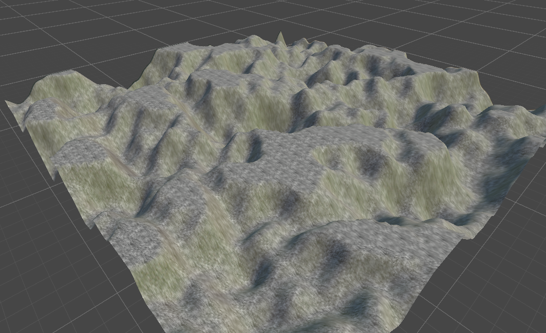
The terrain already resembles a savanna-type land from a satellite image from the sky, but real terrain is often more detailed and varied in places such as mountains, hills, valleys or weathered rivers. Small ridges, slopes, dents and other finer details need a more sophisticated technique, one of which is fractal Brownian motion (used in my website here for stylistic purposes). It involves adding higher-frequency details with lower amplitude, retaining finer details with lower impact as it is in real life. Where larger features such as walking humans cause a dominant desire path, with small features adding details.

Here $A$ sets the initial amplitude, $G$ reduces it between layers, $L$ increases the frequency, and $R$ rotates the input. The layers are called octaves because their frequencies commonly double.

Surface normals

Lighting the height surface needs a surface normal at every point and uses finite differences to estimate the height a short distance away along $x$ and $z$, then uses the differences to estimate both slopes with the sampling distance $\epsilon$. A large value misses small surface details, while a small value subtracts nearly equal floating-point numbers. Every additional sample also evaluates the complete stack of octaves again.

Gradient noise uses a smooth interpolation polynomial. An example is

with derivative

The derivative is sent through the same interpolations as the noise and produces the height $f$ and its partial derivatives in a single run. For a surface defined by $y=f(x,z)$, the normal is

An analytical derivative gives the higher frequency detail without requiring a separate value of $\epsilon$.

Coasts, plains, and mountains

The noise discussed so far has a range of $[-1,1]$. But that doesn’t generate a world of its own, and we’d need to scale it to make a useful world. For a simplified world starting at $Y=0$, with a maximum build limit of $2W$, $(\operatorname{noise}+1)W$ creates the most trivial possible world. But this leaves little control over the heights of mountains and depth of lakes. It is much more aesthetically pleasing for a world to have tall mountains with varied features than a deep ocean, where complex features are generally absent. More recent versions of Minecraft, after the Caves & Cliffs update, use multiple noise layers and splines to generate another range, providing granular local control which a linear mapping of noise loses.

Newer versions thus use three parameters, continentalness ($C$), erosion ($E$), and peaks and valleys ($PV$). The noise fields now choose a position on the spline, while the spline determines the final height. Erosion changes the height along another dimension of the same mapping, allowing inland terrain to become a plateau without applying the same transformation to the ocean floor, and allowing differentiation between upward and downward styles of terrain due to the asymmetry in how these features form in nature.

Density fields and caves

The current model has a single $y$ value generated for any $(x,z)$. This generates a surface, which might be appropriate for some worlds, but the real world is better modelled as a 3D object, with caves and cliffs (one has a pocket of space and the other a band of not-space).

Representing the world as a 3D sampling space with $d=f(x,y,z)$ and later extracting a mesh after sampling leaves us with a 3D object. Sampling across another dimension does increase the cost of the algorithm, but we can solve this and another problem by using a bias. The real world doesn’t uniformly have chunks of floating rocks due to noise, and similarly we add a vertical bias to encode this fact.

When a known bound on $f$ tells us that $b$ dominates, we can skip computing $f$. Negative $d$ represents pockets of air here.

Another technique used to implement spaghetti caves, like in Minecraft, involves using a narrow band around zeros of the noise.

Whenever the absolute noise value is less than a small number $\tau$, $c$ becomes positive and the location is marked as air. As the surface bends and passes near itself, the resulting tunnels branch and reconnect into interesting patterns.

Fog and soft shadows

Architectural Ruins, a Vision (1798)

Some late-18th-century architectural drawings presented newly completed buildings as ruins. In 1798, Joseph Gandy drew Soane’s newly completed Bank of England how it would be if it was made during the times of the Romans. Atmospheric effects always add a sense of realism and make a simulated object look like something from the real world. To simulate diminishing light intensity along a direction, we use the Beer–Lambert law, where $\rho(t)$ is the density of the fog at point $t$ along the ray.

Constant $\rho$ gives exponential fog.

Treating $\rho$ as a spatial field allows fog to collect in valleys or disappear above a chosen altitude, giving more control over where the fog is concentrated. Separate values for different wavelengths, or primary colours, change the colour of distant terrain, as real light has different coefficients at different wavelengths.

Similarly, using what’s called a signed distance field (SDF), which returns the signed distance to the closest surface, allows the ray to skip empty space before entering the volume. With an exact or conservative distance field, we can step forwards by that distance without passing through the nearest surface. The same representation also gives a useful approximation for soft shadows.

A ray is marched from the surface towards the light while retaining the smallest value of

Here $d(p(t))$ is the distance from the current ray position to the nearest surface, $t$ is the distance travelled from the shaded point, and $k$ controls the softness. A ray which passes close to an obstruction produces a small value and therefore a dark penumbra. Greater clearance produces a larger value and allows more light through. Division by $t$ causes the penumbra to widen as the receiving surface moves farther from the object casting the shadow.

Reducing points on a GPU

A common task in procedural generation, also shared by statistics and graphics, is reducing a large set of objects to a few aggregate values. The renderer needs a bounding box for a set of points, which involves finding the minimum and maximum value along each axis. On the CPU:

for (auto p : particles) {
    min_x = min(min_x, p.x);
    max_x = max(max_x, p.x);
}

GPU threads can coordinate through shared or global memory and synchronization, but coordination leads to worse off performance. A technique called reduction instead compares values pairwise first. For eight values, four comparisons leave four values, then two comparisons leave two, and one final comparison leaves the minimum. The work remains $O(N)$, while the number of stages becomes $O(\log N)$. For four million points, one implementation reduced this step from around $9$ ms on the CPU to less than $0.5$ ms on the GPU.

Ending

This leaves us with a world which only needs to exist when it is being used, and can otherwise remain encoded in its seed.

Authors: Austin Shijo & Sujal Satish Motagi