Graphics Roadmap

Graphics programming deals with the generation and manipulation of images and models. Its primary applications include rendering visuals for movies and games, as well as developing the tools for digital art, image editing, and computer-aided design (CAD), supported by the requisite mathematics. At a high level, the field is often split into two domains: real-time graphics, where performance is critical and images must be generated in milliseconds (e.g., for games and simulations), and offline graphics, where photorealism is the primary goal and render times can be hours or days (e.g., for film and architectural visualization). This roadmap will build the foundations for both, starting with the principles that govern real-time rendering.

From wikipedia,

Some topics in computer graphics include user interface design, sprite graphics, raster graphics, rendering, ray tracing, geometry processing, computer animation, vector graphics, 3D modeling, shaders, GPU design, implicit surfaces, visualization, scientific computing, image processing, computational photography, scientific visualization, computational geometry and computer vision, among others. The overall methodology depends heavily on the underlying sciences of geometry, optics, physics, and perception.

Proficiency in graphics programming requires a strong understanding of foundational concepts and the ability to adapt and implement existing algorithms on new data structures and hardware architectures. Graphics programming also requires a lot of tacit knowledge and is better working in teams.

Prerequisites

Further Resources

Prerequisites

A strong foundation in specific mathematical and programming disciplines is required for proficiency in computer graphics. Weaknesses in these areas will manifest as persistent, hard-to-debug problems.

1) Linear Algebra: This field of mathematics provides the tools to represent and manipulate 3D points, directions, and transformations. For computer graphics, it is essential to build a strong intuition for the geometric effects of its operations. For example, it is crucial to understand how a dot product indicates the angle between two vectors, or how a matrix multiplication can rotate and scale an object. This intuitive grasp is fundamental for correctly building and debugging 3D transformations. A comprehensive theoretical introduction is available via Gilbert Strang’s materials. For a practical approach focused on graphics, the sections related to vectors, matrices, and transformations in Fundamentals of Computer Graphics (HDMD) are essential. A strong command of the following topics is critical:-

Vectors: Operations including addition, subtraction, dot products, and cross products are used for representing positions, directions, and surface orientations.
Matrices: Particularly 4x4 matrices are the standard tool for all geometric transformations. A thorough understanding of matrix multiplication and its non-commutative nature is fundamental.
Transformations: The concepts of translation, rotation, scaling, and projection, and their representation as matrices.

2) Programming Language Proficiency (C++/Rust): Modern graphics APIs are primarily accessed through low-level systems languages. Beyond language syntax, proficiency in debugging is paramount. Graphics bugs are rarely clean crashes; they are often silent, visual errors—a black screen, a corrupted texture, a flickering polygon. Familiarity with debugging tools and methodologies is a prerequisite for making any meaningful progress.

C++: The long-standing industry standard. A good starting point is The Cherno’s C++ Series on YouTube; completing the first 48 videos provides a solid practical foundation for graphics work.
Rust: A modern alternative with strong safety guarantees that prevent entire classes of common bugs. A complete understanding of the concepts in the official Rust book is necessary. After reading, it is recommended to complete the rustlings exercises to solidify understanding. For crate recommendations, see blessed.rs.

Graphics Pipeline

The rendering pipeline is a sequence of logical stages that processes a three-dimensional scene description to generate a two-dimensional raster image. The process can be conceptualized in four major stages.

Scene Definition

This stage involves defining the contents of the 3D scene.

Geometry: Object shapes are primarily represented by triangle meshes. For mathematically smooth surfaces where polygonal approximations are insufficient, primitives like Bezier curves are employed. The management, correction, and optimization of this geometric data is the domain of Computational Geometry.
Animation: For dynamic scenes, Computer Animation techniques are used to deform the mesh’s vertices over time, often through a hierarchical “skeletal” system.

Transformation and Shading Setup

With a static scene defined for a single frame, objects are positioned within the world and their surface properties are defined.

Coordinate Systems and Transformations: A chain of matrix operations based on various coordinate systems is used to transform vertices from their local model space into a final screen representation. Errors in this transformation chain can cause objects to be rendered incorrectly or not at all.
Material and Texture Application: An object’s appearance is defined by its material properties, which are implemented in programs called shaders. Texturing is a common technique used to apply 2D images to a model’s surface to add detail without increasing geometric complexity.

Rendering Execution

This core stage generates the 2D image from the prepared 3D data. There are two principal paradigms for this task.

Rasterization: An efficient, object-order approach where each triangle is projected onto the screen to determine pixel coverage. It is the foundation of real-time graphics due to its performance characteristics. The Software Rasteriser project covers this method.
Ray Tracing: An image-order approach that simulates the physics of light by tracing rays from the camera into the scene to determine what is visible at each pixel. It is used for achieving high photorealism at the cost of performance.

The raw rendered image from the execution stage often undergoes further processing before final display.

Anti-Aliasing: The discrete nature of the pixel grid causes aliasing artifacts (“jaggies”) on diagonal and curved edges. Anti-aliasing techniques are applied to mitigate these artifacts.
Post-Processing: This refers to a series of full-screen shader effects applied to the final 2D image to add cinematic effects such as bloom, color grading, and motion blur.

This roadmap is structured to first build an understanding of the two core rendering philosophies. A mastery of these provides a solid foundation for exploring the other stages of the pipeline in greater detail.

Introduction

Meta-Roadmap

Meta-Roadmap

1a) Software Rasteriser

Software Rasteriser Output
Interactive Software Rasteriser from Sebastian Lague

A fundamental challenge in graphics is translating an abstract 3D model into a concrete 2D image. Imagine a single pine tree, represented in the computer as a list of thousands of triangles, each defined by three points in 3D space. The display screen, however, is just a flat grid of pixels. A systematic process is required to bridge this gap: first, to mathematically project the 3D tree onto the 2D screen as if a camera were taking its picture, and second, to determine precisely which pixels on the grid are covered by each of the tree’s projected 2D triangles.

The core idea for solving this is to approach it methodically, like an artist painting onto a canvas. This approach, known as rasterization, involves taking each 3D triangle from the model, “flattening” it into a 2D shape in screen space, and then systematically scanning the pixel grid to “fill in” the area it covers using a scanline algorithm, which iterates row-by-row across the triangle’s projection. By building a software rasteriser, one implements this entire logical pipeline from scratch on the CPU. This process forces a deep understanding of concepts like barycentric coordinates (the mathematical tool for interpolating data across a triangle’s surface) and clipping (the logic for handling triangles that are only partially on-screen).

This project teaches the classic method of rendering 3D scenes, which forms the basis of most real-time graphics. You will manually implement the pipeline that takes 3D vertices, projects them into 2D space, and fills in the resulting pixels on the screen.

A software rasteriser process geometry and renders the output to screen, as raster data(image/, buffer data). Without a subgroup being explicitly mentioned, if a software is called software rasteriser, it tends to be a cheap and resource efficient rasteriser which heavily approximates physical reality by clever techniques. During its development, you’ll likely encounter and implement basic lighting and shading models such as Ambient, Diffuse, and Specular (like Phong or Blinn-Phong) to give surfaces a sense of depth and interaction with light. Writing a software rasteriser motivates the neccesity for GPU based APIs like openGL, vulkan, Metal, directX and webGPU. Ideally, it’s better to implement features by thinking from first principles and I’d recommend Sebastian Lague for the same, and look around for algorithms from wikipedia or from HDMD book (see Links section). Another comprehensive source is the Tiny Renderer Wiki.

1b) Pathtracer

Path Tracer Output
Path Tracer

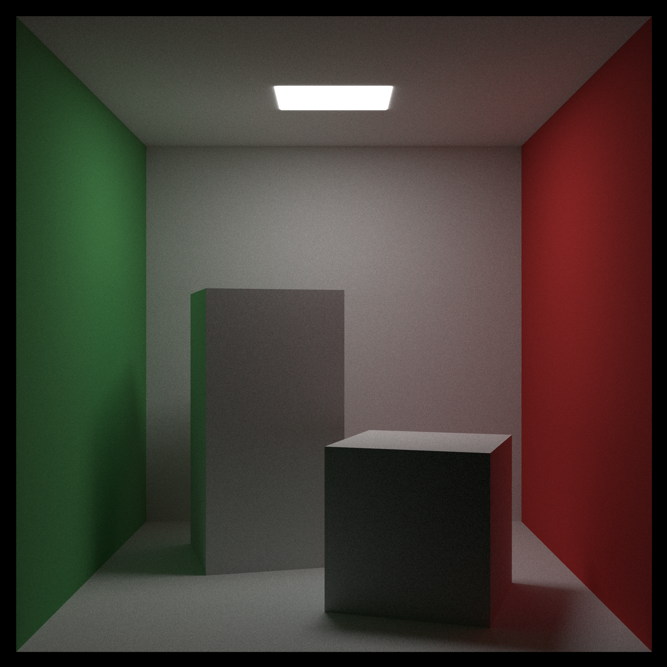
A rasteriser can draw a forest, but the lighting looks artificial. In a real forest, sunlight filtering through a canopy creates soft, dappled light, and the green leaves cast a subtle green hue on the tree trunks below them (color bleeding). The problem is that these are global effects resulting from light bouncing multiple times, whereas basic rasterization only considers the direct path from a light to a surface. A more physically accurate model of light is needed to capture this realism.

The intuition of path tracing is to abandon the “painting shapes” approach and instead simulate the physics of light transport. Rather than asking “which pixels does this triangle cover?”, this method asks “what light would have arrived at this pixel?”. It answers this by tracing a path backwards from the camera into the scene and following it as it bounces between surfaces. Because this is a statistical, random sampling process (a Monte Carlo method), a single sample per pixel is meaningless. The core challenge becomes one of convergence: firing many random rays per pixel and averaging their results to reduce the initial noise into a clean, stable image. The trade-off is a massive increase in computation time for a huge leap in realism.

This project introduces a physically-based approach to rendering that simulates how light actually works. The core idea is to trace the path of light rays recursively. For each pixel, a ray is sent from the camera into the scene. When it hits an object, it bounces off in a new direction, and this process repeats. The final color of the pixel is determined by accumulating the light gathered along this entire path, resulting in highly realistic global illumination, soft shadows, and reflections.

A lot of software rasterisers tend to be raytraced, but another subset of raytraced programs are pathtracers which keep following the path of light throughout. A good motivation to pathtracer is this video until about 10:00. Similarly, I’d recommend following the Sebastian Lague video to implement your own pathtracer and you could read the Ray Tracing in A Weekend to understand how you could potentially design the codebase.

2) GPU APIs

A software rasteriser executing on a CPU processes tasks serially. For a dense forest scene with thousands of trees, this is really slow. Interactive applications require a minimum of 60 frames per second. The fundamental problem is that the CPU, a general-purpose processor, is not designed for the millions of simple, repetitive, and independent calculations inherent to graphics. A specialized parallel processing architecture is needed.

The solution is to offload the work to the Graphics Processing Unit (GPU), a highly parallel processor. A Graphics API (like OpenGL or Vulkan) provides the standardized communication protocol to send instructions and bulk data to the GPU. When using a modern explicit API like Vulkan, the developer takes on several core responsibilities: explicit memory management (allocating buffers on the GPU and uploading data), synchronization (using primitives like fences and semaphores to prevent the CPU and GPU from tripping over each other), and the creation of command buffers (recording sequences of rendering commands to be submitted to the GPU for execution).

These APIs are the interface between your program and the graphics hardware. Learning one is necessary to move beyond the performance limits of software rendering and create complex, high-speed applications.

Once the limitations of software rendering become apparent, especially in terms of performance for complex scenes, the next step is to learn a graphics API that allows you to use dGPUs better. While your software rasterizer implemented the logical stages of a pipeline, a GPU API gives you control over the physical hardware pipeline. For a definitive, low-level explanation of what this hardware is actually doing, read Fabian Giesen’s series, A Trip Through the Graphics Pipeline. It’s an essential resource for understanding the “why” behind API design and performance.

OpenGL: Old, cross-platform API. A good starting point is LearnOpenGL. It provides comprehensive tutorials from basic setup to advanced techniques. openGL is likely a good starting choice but is already deprecated in macOS and is only supported via a translation layer.
Vulkan: A more low-level, explicit API offering more control over the GPU, but with a steeper learning curve. The official Vulkan Tutorial and vulkano for Rust users are good resources. Vulkan generally tends to be more hard-core and is really hard to write manually. It was never implemented for macOS and instead depends on translation layers like moltenVK.
Metal: Apple’s graphics API for macOS and iOS. Apple’s own Metal documentation are the primary resources. Only works for macOS.
WebGPU: An emerging API aiming to bring modern graphics capabilities to the web. The WebGPU specification and sotrh’s learn-wgpu tutorial are recommended. The rust implementation of webGPU, wGPU is the most natural option to use webGPU.

Understanding the rendering pipeline concept is important when working with these APIs. Most APIs abstract this pipeline, but knowing the stages (vertex processing, rasterization, fragment processing, etc.) helps in understanding how graphics are generated and the earlier written projects/techniques motivate the usecase.

While it might seem verbose to write hundreds of lines of code just to draw a triangle, this verbosity stems from the direct control these APIs provide. High-level abstractions like UI toolkits are convenient, but they are built for general-purpose cases and can introduce performance bottlenecks. For example, a generic toolkit might not efficiently batch draw calls; it could end up telling the GPU to draw each button, icon, and text label as a separate operation. This constant back and forth between the CPU and GPU, along with frequent state changes (like swapping shaders or textures for different elements), creates significant overhead.

In a high-performance application like the Zed editor, writing custom renderer allows batching all compatible UI elements into a single draw call and implement custom techniques like SDF-based text rendering, which requires direct control over shaders and data pipelines. This is a level of optimization a generic toolkit cannot provide. Their approach is detailed in their blog post, videogame.

Core Graphics Concepts

These are the universal building blocks used across all other topics. A solid grasp of these concepts is required for any serious graphics work.

3) Coordinate Systems and Transformations

A 3D artist typically creates a model, such as a tree, in its own standardized local space, often centered at the origin (0,0,0). To build a forest, this tree must be placed in a larger world space. This entire world must then be transformed into the view space relative to a camera. Finally, this view is mathematically squashed by a projection transformation into clip space, a canonical cube, before being mapped to 2D pixel coordinates in viewport space. Using assets or code from different systems without a proper conversion matrix will result in objects appearing mirrored.

The intuition is to use a sequential application of 4x4 matrices to represent each step. A model matrix transforms the tree from its local space into the shared world space. A view matrix transforms the world into the camera’s frame of reference. A projection matrix applies perspective. This chain of transformations is fundamental to all 3D rendering, converting geometry from its authored space into a final image.

This is the grammar/syntax of 3D space. It covers how to place, orient, and view objects within a scene using the mathematics of linear algebra.

Understanding different coordinate systems (model, world, view, clip, screen) and the transformations (translation, rotation, scaling, projection) between them is essential. This is where your linear algebra knowledge will be heavily applied. HDMD (see Links section) and scratchapixel both cover these topics well.

4) Shaders

Early fixed-function pipelines (older, non-programmable hardware with a rigid set of rendering capabilities) offered limited control over surface appearance. The problem was a lack of flexibility; to change a lighting calculation, one had to wait for new hardware. A method was needed to allow developers to programmatically define the appearance of materials and create custom visual effects.

The breakthrough was to make the graphics pipeline programmable. Shaders are user-written programs uploaded to the GPU. The intuition is to give the developer direct control: a vertex shader runs for every vertex, allowing for custom transformations, while a fragment shader runs for every pixel of a rendered triangle, allowing for complete control over its final color. This code isn’t run directly; it’s compiled into a hardware-agnostic bytecode like SPIR-V or DXIL, which is then compiled by the GPU driver into native hardware instructions.

Shaders make modern graphics programmable. They are programs that run directly on the GPU, giving you control over how geometry is positioned and how pixels are colored. All modern visual effects are created with shaders.

Shaders are programs that run on the GPU, allowing for programmable control over different stages of the rendering pipeline.

Vertex Shaders: Process individual vertices, typically performing transformations.
Fragment (or Pixel) Shaders: Determine the color of individual pixels/fragments.
Geometry Shaders: Can create or modify primitives which are later processed.
Compute Shaders: For general-purpose computation on the GPU (GPGPU).

You might need to pick a shading language like GLSL (for OpenGL/Vulkan), HLSL (for DirectX), MSL (for Metal), or WGSL (for wGPU). A newly emerging API is Slang which compiles to others easily and is very similiar to HLSL. It supports all features of HLSL and builds and allows transpiling to any lower API. Certain API, webGPU especially requires disabling certain safety features though, although it is equivalent to using unsafe.

5) Texturing

A 3D mesh can define the shape of a tree trunk, but modeling the intricate bark pattern with polygons is computationally infeasible. The problem is how to add this visual detail without increasing the geometric load, which is often a primary performance bottleneck.

The core idea is to decouple visual complexity from geometric complexity through texturing. The intuition is that for any point on the 3D surface, a shader can calculate a corresponding 2D coordinate (UV coordinate) and look up information from an image (texture). A critical aspect of this is filtering. When a textured surface is viewed at an oblique angle, like a road stretching to the horizon, standard filtering causes blurring. Anisotropic filtering is a more advanced technique that samples the texture in a shape that matches the pixel’s projection on the surface, preserving detail at sharp angles.

Texturing provides surface detail, turning simple geometric shapes into believable objects. It involves applying 2D images and other data onto 3D models.

Texture Mapping & UV Coordinates: Mapping 2D images over 3D models.
Filtering & Mipmapping: Reduces aliasing, improves quality at different distances/angles. (Bilinear, trilinear, anisotropic). Mipmaps are pre-scaled texture versions.
Maps:
- Normal Maps: Fake high-res detail on low-poly models. (Polycount Wiki).
- Ambient Occlusion (AO) Maps: Pre-calculate soft shadows for depth. (Polycount Wiki).
- Others (Roughness, Metallic, Height): Crucial for PBR.
Procedural Texturing: Generate textures algorithmically (e.g., noise functions). Infinite variation. (Inigo Quilez’s articles).
PBR Texture Authoring: Create textures describing physical material properties (albedo, metallic, roughness). Needed for modern realism. (Adobe Substance 3D Tutorials, Marmoset guides).
Texture Compression: Reduces memory/storage (BCn, ASTC, ETC). Vital for performance. (NVIDIA Texture Compression Resources, Khronos KTX (Texture Format Standard)).

Advanced Concepts

These topics build on the core concepts to solve more complex problems in geometry, rendering, and simulation.

6) Bezier Curves and Surfaces

When using a vector graphics tool like Inkscape or Photoshop to draw a path, a user needs to create an editable, perfectly smooth curve. Representing this curve with a series of tiny straight lines (a polygonal chain) called polyline would appear jagged at high magnification and would be difficult for the user to manipulate intuitively and precisely. A mathematical representation for smooth curves that is both efficient to store and easy to edit is required.

The intuition is to define a curve not by the points that lie on it, but by a set of control points that guide its shape. Bezier curves use a polynomial function to generate a perfectly smooth path that is influenced by these control points. This allows artists and designers to easily and intuitively create and modify complex, smooth shapes by simply moving a few control points, with the curve itself being calculated by the machine.

These are mathematical descriptions for smooth curves and surfaces, controlled by a set of points. They are essential in any application that requires non-polygonal shapes.

Bezier curves and surfaces are parametric curves and surfaces frequently used in computer graphics for designing smooth shapes and paths like in graphics editors and games for paths (movement of cameras and so on). They are defined by a set of control points and are foundational in vector graphics, font design, and modeling smooth organic forms. For an extremely comprehensive but accessible explanation, pomax which covers everything from the mathematical foundations to practical implementation details. Beauty of Bezier Curves tends to be a less comprehensive introduction to intuition behind Bezier Curves.

7) Computational Geometry

In a large-scale simulation, such as a forest fire, the system must determine which of the thousands of trees are currently touched by the spreading flames. A brute-force check of every triangle of the fire against every triangle of every tree would be computationally impossible due to the combinatorial explosion of checks required. The problem is one of complexity: a more intelligent method is needed to rapidly reduce the number of expensive intersection tests that must be performed.

Computational Geometry (CG) is a foundational repository of knowledge that provides algorithms to solve such problems. The intuition is to use simplified spatial queries to cull the search space. For example, instead of detailed triangle checks, the simulation can first perform cheap intersection tests on the convex hulls—the simplest convex shape enclosing an object—of the trees and the fire. Only if these simple hulls intersect is the more expensive per-triangle check performed. As detailed by resources like Wikipedia, CG also provides fundamental processes like triangulation (breaking complex polygons into triangles) and shape fitting (finding the smallest bounding box for a mesh), which are critical preprocessing steps for building efficient spatial data structures like Bounding Volume Hierarchies (BVHs).

This field provides the algorithms needed to query and manipulate geometric data. It’s the theory behind practical problems like checking if two objects are intersecting or simplifying a complex model.

This field deals with algorithms for defining, manipulating, and analyzing geometric shapes. It’s fundamental for tasks like collision detection, mesh processing, and procedural modeling. O’Rourke’s Computational Geometry in C is a good book explaining both the theory and C implementations of many core algorithms. For video lectures, see CMU’s DDG course.

8) Discrete Differential Geometry (DDG)

To realistically simulate how a character’s cape flows in the wind, the simulation needs to model physical properties like the fabric’s resistance to bending. These concepts are defined by the mathematics of differential geometry, which applies to smooth, continuous surfaces. A method is needed to adapt these powerful mathematical tools to the cape’s representation as a simple, non-smooth triangle mesh.

The core idea of Discrete Differential Geometry (DDG) is to find discrete, mesh-based equivalents for the concepts of smooth geometry. It reformulates properties like curvature and derivatives in a way that is compatible with the simple vertex-edge-face structure of a mesh, enabling advanced physical simulation and shape analysis on standard polygonal models.

DDG applies the mathematics of smooth surfaces (differential geometry) to the discrete triangle meshes used in graphics. This enables sophisticated analysis and manipulation of geometry, such as simulating how a surface deforms.

DDG focuses on applying concepts from differential geometry to discrete surfaces like triangle meshes. It’s crucial for advanced mesh processing, geometry analysis, and developing shape deformation and simulation techniques. Keenan Crane’s DDG course at CMU (Discrete Differential Geometry Course) is a good reference.

9) Real-Time Rendering

Rendering a dense forest at 60 frames per second requires managing strict rendering budgets for each stage of the pipeline (e.g., a 2ms budget for shadows, 1ms for post-processing). A physically-based path tracer would exhaust this budget thousands of times over. The central problem of real-time graphics is to create the most convincing illusion of realism using a limited set of computational resources.

The intuition of real-time rendering is to develop a lot of approximations. This entire field, as catalogued in resources like the Real-Time Rendering book, is a study in trade-offs. For example, deferred shading is a technique that decouples lighting from geometry, making it efficient to render many lights, but the trade-off is higher memory usage for the G-buffer (a set of full-screen textures storing geometric data) and difficulties with transparency. The goal is to choose the right set of techniques and approximations to achieve the desired visual quality within the performance budget.

This area focuses on generating images at interactive frame rates (e.g., 60 FPS) for applications like games and simulations where speed is critical.

This section focuses on techniques for generating images at interactive frame rates, the kind you need for games and simulations. The essential resource here is the book Real-Time Rendering. This book is less of a step-by-step tutorial and more of a “second reading”. Once you’ve learned a concept from another resource, you can read this book to see how it can be implemented, optimized, and pushed to its limits for performance. It covers of state-of-the-art methods and the clever hacks used to make things run fast. As you may have noticed, graphics books repeat the same basics endlessly; get used to it. This book is where you go for the material that comes after the basics.

Deferred Shading: A technique that separates geometry rendering from lighting. First, you render all the scene’s data into a set of textures called a G-buffer (or Geometry Buffer, which stores data like position, normals, and color for every pixel on the screen). Then, a single screen-space shader processes this buffer to calculate all the lighting. This is highly efficient for scenes with many dynamic lights because you decouple lighting from geometry.
Shadow Algorithms: Techniques like Shadow Mapping, where the scene is rendered from the light’s point of view to create a depth map, and its many, many variants (cascaded shadow maps, variance shadow maps) exist to solve its various artifacts and limitations.
Real-Time Global Illumination: True GI is too expensive for real-time, so it has to be approximated. It includes techniques such as Screen-Space Ambient Occlusion (SSAO), which darkens creases, cracks, and corners to fake the soft shadows that result from indirect lighting, adding a great deal of depth to a scene for a relatively low performance cost as it can be run purely on GPU.
Anti-Aliasing: Getting rid of jagged edges (“jaggies”) is crucial. The book details the evolution of techniques from traditional Multisample Anti-Aliasing (MSAA) to modern post-processing methods like Fast Approximate Anti-Aliasing (FXAA) and Temporal Anti-Aliasing (TAA), which leverages information from previous frames to produce a smoother image.

10) Post-Processing

The direct render of a sunlit forest at noon might look harsh and sterile. To create the atmospheric effect of a hazy morning, the bright sun needs a glowing bloom effect around it, and the overall colors of the scene need to be shifted towards a cooler, desaturated palette via color grading. These are effects that must be applied to the entire image globally, not to individual objects within the scene.

The intuition behind post-processing is to treat the entire rendered scene as a single 2D image that can be manipulated. The process involves rendering the scene not directly to the screen, but to an intermediate texture. Then, that texture is drawn to fill the screen, and a special fragment shader is used to apply filters like blurring, color shifting, or adding glow, treating the original rendered image as input data.

Bloom
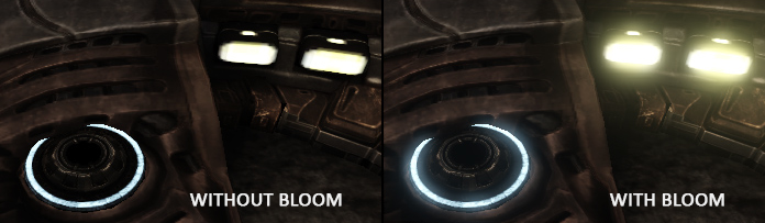
Bloom

Tone Mapping

DOF
Depth of field

Common techniques include:

Bloom: Creates a glowing halo effect around bright areas of an image.
Tone Mapping: Converts High Dynamic Range (HDR) color values into a range suitable for standard displays.
Color Grading: Adjusts the colors of the final image to establish a mood or artistic style.
Depth of Field (DoF): Simulates a camera lens by blurring parts of the scene that are out of the focal plane.
Motion Blur: Blurs objects based on their velocity to create a sense of speed and smooth animation.

Resources:

The Post Processing chapter on LearnOpenGL provides a practical implementation guide.
The Cherno’s video on Bloom explains the concept and implementation.
John Hable’s blog post is a classic resource on filmic tone mapping.

11) Anti-Aliasing

no SSAA	SSAA

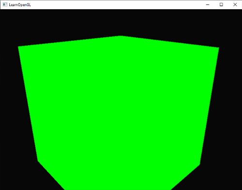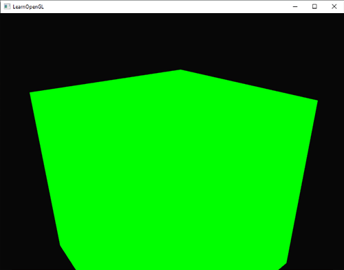The process of representing a continuous, smooth edge—like the silhouette of a distant mountain against the sky—on a discrete, square pixel grid creates a visually jarring “staircase” effect. This artifact, known as aliasing, makes rendered images look sharp, artificial, and shimmer distractingly when the camera or objects are in motion. A method is needed to soften these edges and create a more natural appearance.

The core idea of anti-aliasing is to avoid a binary “in or out” decision for pixels that lie on a triangle’s edge. Instead, it calculates a partial coverage value. A pixel that is 30% covered by a foreground object and 70% by the background will be colored with a 30/70 blend of their respective colors. This blending creates a smoother visual transition that is less jarring to the eye. Below are common approaches with their trade-offs.

Supersampling (SSAA): The brute-force, highest-quality approach. It renders the entire scene at a much higher resolution and then downscales it. The enormous performance cost makes it unsuitable for most real-time applications.
Multisample Anti-Aliasing (MSAA): A hardware-based optimization that only supersamples the pixels on the edges of polygons. It provides good quality for geometric edges at a reasonable cost but fails to fix aliasing from textures or shaders and is often incompatible with deferred rendering.
Post-Process Anti-Aliasing (e.g., FXAA): A shader that runs on the final image to detect and blur jagged edges. It is very fast and compatible with all rendering pipelines, but the trade-off is a potential for noticeable blurring across the entire image.
Temporal Anti-Aliasing (TAA): The modern standard. It reduces aliasing by blending the current frame with reprojected data from previous frames. It is highly effective but can introduce “ghosting” or smearing artifacts on fast-moving objects.

This is the process of smoothing the jagged edges that result from rasterization. The correct technique to use depends entirely on the context, such as performance constraints or the type of geometry being rendered.

Anti-aliasing reduces jagged edges from rasterization. The optimal technique depends on the use case. This article on Analytical Anti-Aliasing covers several methods.

The article reviews sampling-based approaches like SSAA (Supersampling) and MSAA (Multisample Anti-Aliasing), explaining their function and performance costs. It uses this context to introduce Analytical Anti-Aliasing (AAA).

AAA is not a general-purpose replacement for other methods. It is for primitives with a mathematical definition, such as lines or circles. Instead of sampling, AAA calculates the exact geometric coverage of the primitive within a pixel. This is effective for rendering vector graphics or UI elements, where it produces clean edges without the blur of post-processing filters or the high cost of supersampling.

For general 3D scenes, MSAA or TAA are common. For vector-based graphics, AAA is often a better choice.

12) Offline Rendering

For applications where visual fidelity is the only priority and render time is not a constraint, such as in cinematic visual effects, the approximations of real-time rendering are insufficient. A methodology is needed that does not compromise on quality and instead attempts to solve the full, complex problem of how light behaves in a physical space, however long the computation takes.

The intuition of offline rendering is to fully simulate the physics of light as described by the Rendering Equation. Instead of cutting corners for speed, these techniques use advanced statistical methods (like Monte Carlo integration) and complex light transport algorithms to find the most accurate possible solution. The focus shifts entirely from performance to physical correctness, as exemplified by comprehensive systems described in texts like Physically Based Rendering (PBRT).

This is the domain of film and visualization, where visual quality and physical accuracy are the only priority, and performance is secondary. The goal is to solve the Rendering Equation, which describes the physics of light.

Where real-time rendering is about speed, offline rendering is about uncompromising quality. This is the domain of film, architectural visualization, and scientific simulation, where taking several minutes to render a single frame is acceptable to achieve physical accuracy. The theoretical backbone for this entire field is the Rendering Equation, which mathematically describes how light moves around in a scene. While you can’t “solve” it directly, all the techniques below are attempts to get as close as possible.

The best resource for this topic is Physically Based Rendering: From Theory to Implementation (PBRT). It’s not just a book; it’s a complete, production-grade renderer written in a “literate programming” style, meaning the book is the source code. If you want to understand how these systems are built from the ground up, this is your bible.

As you work through it, you’ll encounter these core ideas:

Global Illumination (GI): This is the main goal. It’s about simulating not just direct light from a source, but also the indirect light that bounces off other surfaces. This is what gives you soft shadows and color bleeding (e.g., the red tint a carpet casts on a white wall).
Light Transport Algorithms: These are the strategies for simulating light bounces. The workhorse is Path Tracing, which traces random light paths from the camera. For more complex lighting scenarios, like caustics from a glass of water, more advanced methods like Bidirectional Path Tracing (tracing from both the camera and lights) or Metropolis Light Transport (which searches for important light paths) are used.
Participating Media: For rendering things that aren’t solid surfaces. Think fog, smoke, clouds, or murky water. This involves simulating light getting absorbed or scattered as it travels through a volume.
Subsurface Scattering (SSS): Crucial for translucent materials. It’s how you get the soft, characteristic look of skin, wax, or marble, where light enters the object, scatters around inside, and exits at a different spot.

13) Volume Rendering

Standard graphics techniques are designed to render the surfaces of objects. They are unsuitable for phenomena that have no distinct surface but exist throughout a 3D space, such as the morning fog hanging in a forest valley or the complex, puffy structure of a cloud. A different rendering approach is needed for these volumetric phenomena.

The intuition of volume rendering is to work with data that exists in a 3D grid (voxels) or is defined by a mathematical function, instead of a 2D surface (triangles). The primary method, ray marching, involves stepping a ray through this 3D grid, sampling the data (e.g., fog density) at each step, and accumulating color and opacity along the ray’s path to form a final pixel color. For generating the cloud shapes themselves, a procedural noise function can define the density, and an algorithm like marching cubes can be used to extract a mesh-like surface from that density field if needed.

This topic covers the visualization of data that occupies a 3D space, rather than just existing on a 2D surface. It is essential for medical imaging and scientific simulation where seeing the inside of an object is necessary.

Volume rendering is used to visualize data that exists within a 3D space, rather than just on surfaces, making it critical for medical imaging (CT/MRI scans) and scientific visualization. It operates on a 3D grid of data points called voxels. There are two main approaches.

The first, direct volume rendering, uses ray marching to step a ray through the volume, sampling the data and accumulating color and opacity at each point. A transfer function is key here, as it maps data values (like tissue density) to visual properties, allowing you to “see through” the data. The book Real-Time Volume Graphics is a comprehensive resource for this. For a practical, shader-based implementation, see the tutorial on GPU-based raycasting and Inigo Quilez’s work on rendering worlds with distance functions.

The second approach is indirect, using an algorithm like marching cubes to extract a specific surface of constant value (an isosurface) and convert it into a standard triangle mesh. This is perfect for creating a solid model of a particular feature, like a bone from a CT scan, which can then be rendered with normal rasterization techniques. The definitive text is the original 1987 SIGGRAPH paper: Marching Cubes: A High Resolution 3D Surface Construction Algorithm. For a more accessible explanation of the implementation, refer to Paul Bourke’s article. The choice depends on the goal: use ray marching to see semi-transparent and interior structures, or use marching cubes to extract a clean, solid surface from the data.

14) Text Rendering

Rendering text for a user interface appears simple but is a highly specialized domain. The challenges include parsing complex binary font files, converting the vector-based letter outlines into sharp, readable pixels at any size, and correctly applying complex typographic rules for layout, such as kerning and ligatures.

The solution is to treat text rendering as a multi-stage pipeline. A font parsing library reads the glyph data from the font file. A rasterization technique then converts the vector shapes to a texture; modern approaches use Signed Distance Fields (SDFs) for high-quality, scalable results. Finally, a layout engine positions the rasterized glyphs from this texture according to typographic rules.

This is a specialized domain focused on correctly parsing font files, converting glyphs into pixels, and arranging them into legible words and sentences.

Text rendering is a complex domain. The process involves more than rendering glyphs to the screen.

The process begins with parsing font files (like .ttf or .otf), which contain glyphs defined by Bezier curves.
These vector outlines then need to be rasterized into pixels. A common approach is to pre-rasterize them into a texture atlas.
A more advanced and flexible method is using Signed Distance Fields (SDFs). Instead of storing the pixel color, the texture stores the distance to the nearest glyph edge. This allows for scaling text smoothly without it becoming pixelated or blurry, as the shape can be reconstructed in the shader. Sebastian Lague has a great video explaining the concept.
Finally, text layout addresses the complexities of arranging characters correctly. This involves kerning (adjusting the space between specific pairs of letters like ‘A’ and ‘V’), handling ligatures (combining characters like ‘f’ and ‘i’ into a single ‘fi’ glyph), and supporting complex scripts like Arabic or Hindi, which requires sophisticated shaping logic. Libraries like FreeType and HarfBuzz are often used to handle this complexity.

15) Computer Animation

A 3D model of a deer is a static, lifeless sculpture. To make it walk through the forest, a system is needed to deform its mesh over time in a structured and controllable way. Similarly, to bring the environment to life, the thousands of trees in the forest should appear to sway in the wind, which requires applying a subtle, coordinated motion to a vast number of objects at once.

The intuition for character motion is skeletal animation, where an internal “skeleton” of bones deforms the mesh, allowing for complex, articulated movement. An alternative for subtler deformations like facial expressions is blend shapes (or morph target animation), which interpolates the entire mesh between different pre-sculpted poses. For environmental motion like swaying trees, the intuition is often procedural animation, where a mathematical function is used in a shader to generate motion on-the-fly.

This section covers techniques for creating the illusion of movement by transforming geometry over time.

Animation is fundamentally about transforming geometry over time.

Skeletal Animation: This is the standard technique for character animation. It involves creating a hierarchical skeleton of “bones” (a rig) and attaching the mesh’s vertices to them with varying influence weights (skinning or vertex blending). The animation is then driven by rotating the bones in the rig. Animators can control this using Forward Kinematics (FK), where they set the angle of each bone directly, or Inverse Kinematics (IK), where they position an end-effector (like a hand or foot) and the algorithm calculates the required bone rotations to reach it.
Physics-Based Simulation: Physics-based techniques are employed for more dynamic and realistic motion. This includes simulating cloth using mass-spring systems or position-based dynamics, simulating hair and fur, and fluid dynamics for water and smoke using complex mathematical models like the Navier-Stokes equations.
Keyframing and Procedural Animation: Keyframing is the manual process where an animator sets key poses at specific frames, and the computer interpolates the motion between them. Procedural animation, on the other hand, generates motion algorithmically, which is useful for complex systems like flocks of birds or crowds. A good motivator is this t3ssel8r’s video on mathematical procedural animation and argonaut’s video on constraint based procedural animation.

16) Procedural Generation

Manually authoring vast amounts of content, such as an entire planet’s worth of terrain, millions of unique trees, or the detailed shapes of clouds, is a prohibitively labor-intensive task. An algorithmic approach is needed to generate this content at scale while maintaining a natural, non-repeating appearance. The main challenge is not simply generating randomness, but creating systems that are art-directable, allowing designers to control the style and key features of the generated world.

The intuition of procedural generation is to replace manual artistry with algorithms that use controlled randomness. A noise function, for example, can generate natural-looking, random-yet-structured values. This noise can be used to define the height of the terrain, the density of trees, or the 3D density field for clouds which can then be rendered using volume rendering techniques. This allows a computer to generate vast and unique worlds from a small set of rules.

This is the practice of using algorithms to create data rather than creating it manually. It is used to generate content ranging from textures to entire game worlds.

Procedural generation is the algorithmic creation of data. This field encompasses a wide range of applications, from generating textures with noise functions to creating entire game worlds.

Noise Functions: Algorithms like Perlin noise, Simplex noise, and Worley noise are fundamental. They produce natural-looking, pseudo-random patterns that are used for creating textures like wood, marble, clouds, and for generating terrain heightmaps.
L-systems (Lindenmayer systems): These are rewriting systems and a type of formal grammar. They are often used for generating fractal structures, especially for modeling the growth of plants, trees, and other branching structures.
Shader-Based Generation: Using fragment shaders to generate complex visuals in real-time. The articles by Inigo Quilez are a highly-regarded resource for shader-based procedural generation, especially using signed distance functions to model shapes.
World Generation: This can involve using fractal noise to generate terrain heightmaps, and then applying simulation algorithms (like hydraulic and thermal erosion) to make them more realistic.

Further Resources

SIGGRAPH: The premier conference for computer graphics. Papers and courses from SIGGRAPH are a goldmine of information, often available through the ACM Digital Library.
GPU Gems Series: Books containing articles on various advanced GPU techniques.
Graphics Programming Weekly: A newsletter by Jendrik Illner (Graphics Programming Weekly), can help keep you updated with new developments.
Graphics Debugging Tools: Proficiency with a tool like RenderDoc or NVIDIA Nsight is not optional. These tools allow for the capture and frame-by-frame dissection of a graphics application, which is essential for debugging visual artifacts.
Youtube channels: There are plenty of channels which offer open ended theoritical exploration of topics such as Sebastian Lague, acerola.

Contributors

Austin Shijo | @austins24