

Web3 Roadmap

Welcome to the Natural Language Processing Roadmap «»
This roadmap is your hands-on, no-fluff guide to mastering NLP—from basic text processing to implementing actual working code. Over 9 structured weeks, you’ll progressively unlock NLP’s core concepts through carefully designed content, practical mini assignments, and real-world projects. While challenging, everything here is absolutely achievable with consistent effort and curiosity.
Flexible Structure (Highly Recommended but Not Rigid)
We’ve arranged topics in a logical progression, especially for the first few weeks where NLP techniques form the critical foundation.
Timing is flexible too. Some days, you’ll binge a week’s content in one sitting; other times, a single concept might take days to click. Both are normal! The key is to keep moving forward without burning out. Enjoy the journey—NLP is as much art as it is science .
Machine Learning primarily deals with structured datasets—numbers, tables, and well-organized records that can be fed into algorithms.
But what if we want to analyze something more complex? For example, suppose we want to assess a company’s market status by understanding its recent news articles, press releases, or social media updates. These are written in natural language, which is messy, ambiguous, and heavily dependent on context.
This raises the question: How can machines make sense of language—the way humans naturally communicate?
The answer lies in Natural Language Processing (NLP), a subfield of AI that enables machines to process, understand, and generate human language. Through NLP techniques such as text preprocessing, embeddings, sentiment analysis, and language models, we can extract insights from unstructured text data, allowing applications like:
Thus, NLP bridges the gap between raw human language and structured machine understanding, enabling Machine Learning to be applied meaningfully to text-based problems.
This roadmap begins with the foundations of text preprocessing and representation, where we learn to clean, normalize, and encode text using techniques like Bag-of-Words, TF-IDF, one-hot encoding, and word embeddings, eventually leveraging pretrained embeddings for tasks such as sentiment classification. From there, we move into sequence models, starting with RNNs and LSTMs, implementing them from scratch, and then extending to GRUs and statistical language modeling with n-grams, Seq2Seq, and beam search decoding.
Building on this, we introduce attention mechanisms—self-attention, multi-head attention, and scaled dot-product attention—leading to the implementation of a basic Transformer and a deeper exploration of encoder-decoder, encoder-only, and decoder-only architectures. With this foundation, the roadmap transitions into Large Language Models (LLMs), covering their design, visualization, transfer learning, fine-tuning, evaluation, and multilingual applications, followed by advanced reinforcement learning techniques for LLMs such as RLHF, DPO, and multi-agent reinforcement learning.
Finally, we expand into speech and multimodal NLP, where we explore text-to-speech pipelines, neural vocoders, automatic speech recognition (ASR) with models like Whisper and wav2vec, and emerging cross-modal NLP trends, concluding with hands-on projects in TTS, ASR, and multimodal applications.
Remember , small efforts everyday culminate in making a huge impact. Hence don’t feel too overwhelmed by the length of this roadmap . Go day by day and step by step, and you’ll find your knowledge growing immensely.
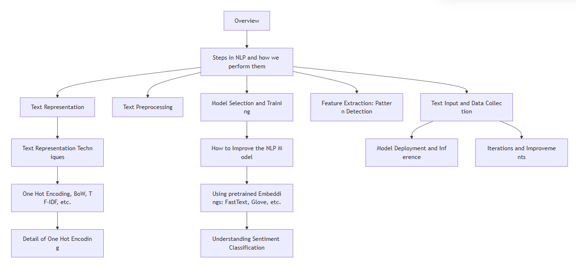
Week 1: Text Preprocessing and Embedding Techniques
Week 2: RNNs, LSTMs and Sequence Modeling
Week 3: GRUs and Language Modelling
Week 4: Attention like that of transformers
Week 5: Deep dive into Transformer Models and Intro to LLMs
Week 6: Large Language Models (LLMs) and Fine-Tuning
Week 7: Advanced Reinforcement Learning Techniques for NLP & Large Language Models
Week 8: Speech and Multimodal NLP
Week 9 : Speech-to-Text & Cross-Modal NLP
First of all, check out this amazing playlist by TensorFlow to get a crisp idea of what we are going to do this week. It’s packed with insightful videos that will lay a solid foundation for your NLP journey!
Concisely speaking , the topics above play the role of Data Sanitization, and are hence extremely important to study NLP. Lets dive deeper below :
Imagine trying to read a messy, smudged book – not fun, right? Text preprocessing is like cleaning up that book, making it crisp and readable. It transforms chaotic, noisy text into a tidy format that’s ready for analysis. This process is crucial because cleaner data leads to better NLP model performance!
Explore More: Dive deeper into text preprocessing here.
Think of text normalization as decluttering your digital workspace. It standardizes text, eliminating noise and focusing on the essence. This involves steps like converting text to lowercase, removing punctuation, and applying techniques like lemmatization and stemming. Essentially, it’s text preprocessing on steroids!
Discover the Magic of Normalization: Learn more about normalization here
Regular expressions (regex) are like the ultimate search-and-replace tool, but on steroids! They help you find patterns in text – imagine being able to pinpoint every email address or phone number in a document with a simple command.
Check out this blog on regex here
Ever wondered how similar two strings are? Edit distance, specifically Levenshtein distance, tells you the minimum number of edits (insertions, deletions, substitutions) needed to transform one string into another. It’s like calculating the steps to turn “kitten” into “sitting.”
Get Detailed Insight: Learn more about edit distance here
a. Bag of Words (BoW): The Basic Building Block Imagine reducing a sentence to a simple bag of words, ignoring grammar and order. BoW does just that, focusing on the presence of words. It’s a straightforward way to tokenize text but doesn’t capture context.
Understand BoW: Explore the concept of Bag of Words here
b. TF-IDF: Adding Depth to Word Representation TF-IDF adds a twist to BoW by weighing terms based on their importance. It highlights significant words while downplaying common ones. TF (Term Frequency) measures how often a word appears in a document, while IDF (Inverse Document Frequency) gauges the word’s rarity across documents.
Formula Breakdown:
Term Frequency (TF):
\[TF(t, d) = \frac{\text{Number of times term } t \text{ appears in document } d}{\text{Total number of terms in document } d}\]Inverse Document Frequency (IDF):
\[IDF(t, D) = \log \left( \frac{\text{Total number of documents}}{\text{Number of documents containing the term } t} \right)\]TF-IDF Score:
\(TF\text{-}IDF(t, d, D) = TF(t, d) \times IDF(t, D)\) Explore More: Get a detailed understanding of TF-IDF here.
CBOW is part of the Word2Vec family, predicting a target word based on its context. It’s like filling in the blanks in a sentence using surrounding words, capturing semantic relationships.
How It Works: For the sentence “The quick brown fox jumps over the lazy dog” and the target word “fox,” CBOW uses the context (“The,” “quick,” “jumps,” “over”) to predict “fox.”
Discover CBOW: Learn more about Continuous Bag of Words here.
Imagine trying to categorize a group of objects where each object belongs to a unique category. One-hot encoding is like assigning a unique ID card to each word in your text, where each card contains just one slot marked “1” and all other slots marked “0.” This approach transforms words into a format that machines can understand and process.
Each word is represented as a vector with a length equal to the total number of unique words (vocabulary size). In this vector, only one element is “hot” (set to 1), and the rest are “cold” (set to 0). Example: For a vocabulary of [‘apple’, ‘banana’, ‘cherry’]: ‘apple’ → [1, 0, 0] ‘banana’ → [0, 1, 0] ‘cherry’ → [0, 0, 1] Explore More: Learn more about one-hot encoding here.
You shall know a word by the company it keeps — J.R. Firth While one-hot encoding is simple, it doesn’t capture the relationships or meanings of words. Enter word embeddings – a more sophisticated approach where words are represented as dense vectors in a continuous vector space. These vectors are learned from the text data itself, capturing semantic relationships and similarities between words.
Word embeddings are created using algorithms like Word2Vec, GloVe, or FastText. Each word is mapped to a vector of fixed size (e.g., 100 dimensions) where similar words have similar vectors. Example: For the words ‘king’, ‘queen’, ‘man’, and ‘woman’, word embeddings might capture the relationships like: ‘king’ - ‘man’ + ‘woman’ ≈ ‘queen’ ‘man’ and ‘woman’ will be closer to each other in the vector space than ‘man’ and ‘banana’. Explore More: Dive deeper into word embeddings here.
Think of pretrained embeddings as getting a head start in a race. Instead of starting from scratch, you leverage the knowledge already learned from massive text corpora. This can significantly boost your NLP models’ performance by providing rich, contextual word representations right out of the box.
Pretrained embeddings, such as those from Word2Vec, GloVe, and FastText, are trained on large datasets like Wikipedia or Common Crawl. These embeddings capture nuanced word meanings and relationships, offering a robust foundation for various NLP tasks. Benefits: Efficiency: Saves time and computational resources since the heavy lifting of training embeddings has already been done. Performance: Often leads to better model performance due to the high-quality, contextual word representations. Transfer Learning: Facilitates transfer learning, where knowledge from one task (like language modeling) can be applied to another (like sentiment analysis).
Description: Unlike Word2Vec and GloVe, FastText considers subword information, making it effective for morphologically rich languages and rare words.
How to Use: Available via the FastText library. Load pretrained vectors and incorporate them into your models with ease.
Explore More: Dive deeper into pretrained embeddings and their applications here.
This is the first real world use case of NLP that we are going to discuss from scratch.
Imagine trying to understand someone’s mood just by reading their messages. Sentiment classification does exactly that – it helps in identifying the emotional tone behind a body of text, whether it’s positive, negative, or neutral. This technique is widely used in applications like customer feedback analysis, social media monitoring, and more. By Definition, Sentiment analysis is a process that involves analyzing textual data such as social media posts, product reviews, customer feedback, news articles, or any other form of text to classify the sentiment expressed in the text.
How It Works: Sentiment classification models analyze text and predict the sentiment based on the words and phrases used.The sentiment can be classified into three categories: Positive Sentiment Expressions indicate a favorable opinion or satisfaction; Negative Sentiment Expressions indicate dissatisfaction, criticism, or negative views; and Neutral Sentiment Text expresses no particular sentiment or is unclear. These models can be built using various algorithms, from simple rule-based approaches to complex machine learning techniques.
Example: For the sentence “I love this product!”: The model would classify it as positive. For “I hate waiting for customer service,” it would classify it as negative. 🎥 Watch and Learn: Learn more about sentiment classification here.
Rule-Based Methods
Description: These methods use a set of manually created rules to determine sentiment. For example, lists of positive and negative words can be used to score the sentiment of a text. Pros: Simple and interpretable. Cons: Limited by the quality and comprehensiveness of the rules. Machine Learning Methods
Description: These methods use labeled data to train classifiers like Naive Bayes, SVM, or logistic regression. The models learn from the data and can generalize to new, unseen texts. Pros: More flexible and accurate than rule-based methods. Cons: Require labeled data for training and can be computationally intensive. Deep Learning Methods
Description: These methods leverage neural networks, such as RNNs, LSTMs, or transformers, to capture complex patterns in the text. Pretrained models like BERT and GPT can also be fine-tuned for sentiment analysis. Pros: State-of-the-art performance, capable of capturing nuanced sentiments. Cons: Require significant computational resources and large amounts of data.
For a detailed walkthrough on sentiment analysis using NLP techniques, check out this comprehensive video tutorial
Sentiment Analysis Video
In this video, you’ll learn about:
thus it will help you revise the whole week of content.
Congratulations on making it through the first week of your NLP journey! Today, we’re going to dive into some beginner-friendly projects to help you apply what you’ve learned. These projects will solidify your understanding and give you practical experience in working with NLP.
Sentiment Analysis on Movie Reviews Objective: Build a model to classify movie reviews as positive or negative. Dataset: IMDb Movie Reviews Tools: Python, NLTK, Scikit-learn, Pandas Steps: Preprocess the text data (tokenization, removing stop words, etc.). Convert text to numerical features using TF-IDF. Train a machine learning model (e.g., logistic regression). Evaluate the model’s performance.
Text Classification for News Articles Objective: Categorize news articles into different topics (e.g., sports, politics, technology). Dataset: 20 Newsgroups Dataset Tools: Python, Scikit-learn, Pandas Steps: Preprocess the text data. Convert text to numerical features using count vectorization. Train a classification model (e.g., Naive Bayes). Evaluate the model’s accuracy and fine-tune it.
Spam Detection in Messages Objective: Create a model to identify spam messages. Dataset: SMS Spam Collection Tools: Python, NLTK, Scikit-learn, Pandas Steps: Preprocess the text data. Feature extraction using count vectorization or TF-IDF. Train a machine learning model (e.g., SVM). Test the model and improve its performance.
Named Entity Recognition (NER) Objective: Identify and classify named entities (like people, organizations, locations) in text. Dataset: CoNLL-2003 NER Dataset Tools: Python, SpaCy Steps: Preprocess the text data. Use SpaCy to build and train a NER model. Evaluate the model’s performance on test data.
Pick one or more of these projects and get started. Don’t worry if you face challenges along the way; it’s all part of the learning process. As you work on these projects, you’ll gain a deeper understanding of NLP techniques and improve your coding skills.
Remember, practice makes perfect. The more you experiment with different datasets and models, the more proficient you’ll become in NLP. Happy coding!
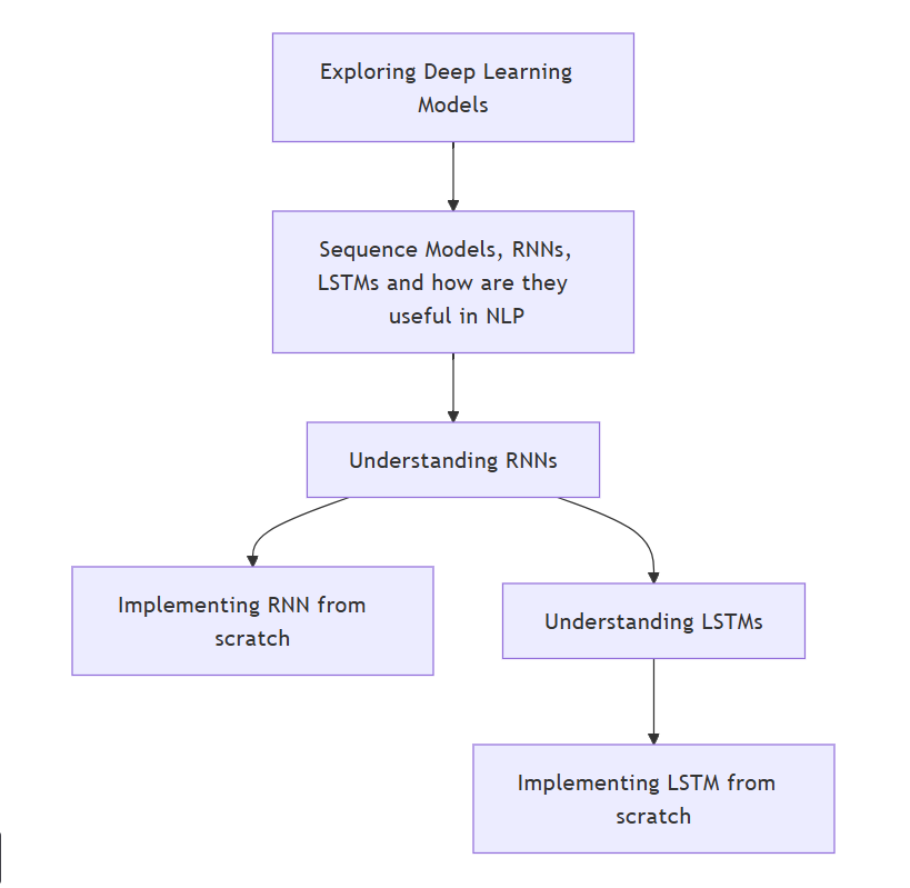
A neural network is a type of artificial intelligence model that maps the structure and function of the human brain to learn from data and make decisions or predictions. It consists of interconnected layers of nodes, or “neurons,” which process information and adjust “weights”(or simply parameters) on their connections to identify patterns and solve complex problems, making them useful for tasks like image recognition, language translation, and predictive analytics.
The core idea here is that language is sequential. It is not a bag of words — its meaning depends on order and context. RNNs/LSTMs are designed to consume a sequence and maintain a hidden state (memory) that summarizes what has come before.
Sequence Models,RNNs and LSTMs are models that process data in a specific order (like sentences or speech). They help machines understand the meaning and context of language by processing words and sentences as sequences, not isolated tokens.
As the name suggests, RNNs are a type of nueral networks that are recurrent in nature . Recurrent here essentially implies that these nueral networks have nodes that linked in a loop. This essentially means that at step pf processing , a node in RNN takes an input and gives an output and this output is provided alongside the input of the next step. This allows the RNN to remember previous steps in a sequence . But RNNs suffer from long term dependency problem which is called so to imply that with time as more information piles up , the RNN fails to learn new things effectively .
Here’s when LSMT comes in to save the day . LSTMs provide a solution to the long term dependency problem by adding an internal state to the RNN node. Now this state information is also used while processing in the node.
Here’s the link to the research paper of the model : Research Paper of RNNs
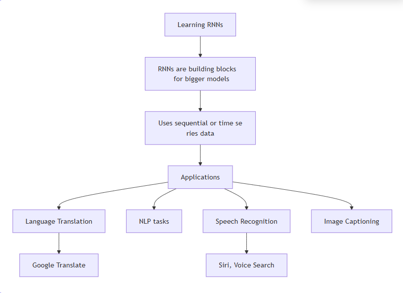
By learning RNN, your journey of NLP with deep learning truly starts here. RNNs by themselves are of little use, but they form the building blocks of many bigger models.
As stated above, a recurrent neural network (RNN) is a type of artificial neural network which uses sequential data or time series data. These deep learning algorithms are commonly used for ordinal or temporal problems, such as language translation, natural language processing (nlp), speech recognition, and image captioning; they are incorporated into popular applications such as Siri, voice search, and Google Translate.
For understanding RNNs and their implementation in tensorflow, go through the following links:
This RNN cheatsheet by Stanford shall come in handy for revision .
While talking about RNNs and LSTMs , context refers memory of past inputs that helps in interpreting the current input correctly.
To truly understand RNNs, you must understand how to implement them from scratch. Use your knowledge to implement them in python, and use the following link as a reference if you get stuck: https://towardsdatascience.com/recurrent-neural-networks-rnns-3f06d7653a85
You can also refer to the following notebooks:
RNNs suffer from issues like vanishing and exploding gradients. To understand these problems in more detail, check out this article:
These issues are largely addressed by Long Short-Term Memory (LSTM) models, which efficiently maintain both short-term and long-term context, while also providing mechanisms to forget information that is no longer needed.
For a deeper understanding of LSTMs, this article is highly recommended:
Use the knowledge gained to implement an LSTM from scratch. You can refer to the following articles if you face issues in implementing it: https://medium.com/@CallMeTwitch/building-a-neural-network-zoo-from-scratch-the-long-short-term-memory-network-1cec5cf31b7
You can also refer to the following notebooks:
There exist various variants and optimized versions of LSTMs and RNNs to better handle sequential data, long-term dependencies, and complex patterns.
Think of reading a sentence : sometimes, the meaning of a word depends on what came before it and what comes after it. This variation processes sequences in both forward and backward directions, allowing the model to capture context from past and future tokens simultaneously.
Uses an encoder-decoder for mapping input sequences to output sequences, commonly used in translation and summarization tasks.
Combines bidirectional LSTMs in the encoder with a decoder, improving context understanding in sequence-to-sequence tasks.
RNNs that read sequences forward and backward, enhancing performance in tasks where both past and future context matter.
Stack multiple RNN layers to learn more complex representations, allowing the model to capture hierarchical patterns in sequential data.
graph TD
  A[ Understanding GRUs]
  B[ Implementing GRUs]
  C[ Statistical Language Model-ing]
  D[ N-Gram Language Models]
  E[ Seq2Seq Models]
  F[ Beam Search Decoding]

  A --> B
  B --> C
  C --> D
  D --> E
  E --> F
Gated Recurrent Unit (GRU) is a type of recurrent neural network (RNN) that was introduced as a simpler alternative to Long Short-Term Memory (LSTM) networks. Like LSTM, GRU can process sequential data such as text, speech, and time-series data. Go through the following articles for better understanding:
To gain better understanding of GRUs, let’s implement it from scratch. Use the following link for reference: https://d2l.ai/chapter_recurrent-modern/gru.html
You can also refer to the following repositories/notebooks:
RNN vs LSTM vs GRU – This paper evaluates and compares the performance of the three models over different datasets.
In NLP, a language model is a probability distribution over strings on an alphabet. Statistical Language Modeling, or Language Modeling and LM for short, is the development of probabilistic models that are able to predict the next word in the sequence given the words that precede it. For a deeper understanding, go through the following resources:
Here’s a paper covering SLM in depth Link
Now that we’ve understood SLMs, let’s take a look into an example of a Language Model: N-Gram. Go through the following resources:
Seq2Seq model or Sequence-to-Sequence model, is a machine learning architecture designed for tasks involving sequential data. It takes an input sequence, processes it, and generates an output sequence. The architecture consists of two fundamental components: an encoder and a decoder. This Encoder-Decoder Architecture is also used in Transformers which we shall study later. Go through these resources for understading Seq2Seq better:
graph TD
  A["Input Sequence"] --> B["Encoder RNN"]
    B --> C["Context / Hidden State"]
    C --> D["Decoder RNN"]
    D --> E["Output Sequence"]

    subgraph Encoder
        B
    end

    subgraph Decoder
        D
    end
Beam search is an algorithm used in many NLP and speech recognition models as a final decision making layer to choose the best output given target variables like maximum probability or next output character. It is an alternative to Greedy Search which is largely used outside NLP, but although Beam Search requries high compute, it is much more efficient than Greedy Search. THis approach is largely used in the decoder part of the sequence model. For better understadning, go through the following:
Attention mechanisms help models focus on relevant parts of input data.
Here’s the link for the paper which introduced the transformer model Attention is all you need
An attention mechanism is a machine learning technique that directs deep learning models to prioritize (or attend to) the most relevant parts of input data. Innovation in attention mechanisms enabled the transformer architecture that yielded the modern large language models (LLMs) that power popular applications like ChatGPT. This mechanism allows the models to weigh the importance of different parts of an input sequence to understand their relationships and context.
As their name suggests, attention mechanisms are inspired by the ability of humans (and other animals) to selectively pay more attention to salient details and ignore details that are less important in the moment. Having access to all information but focusing on only the most relevant information helps to ensure that no meaningful details are lost while enabling efficient use of limited memory and time.
Mathematically speaking, an attention mechanism computes attention weights that reflect the relative importance of each part of an input sequence to the task at hand. It then applies those attention weights to increase (or decrease) the influence of each part of the input, in accordance with its respective importance. An attention model—that is, an artificial intelligence model that employs an attention mechanism—is trained to assign accurate attention weights through supervised learning or self-supervised learning on a large dataset of examples.
RNNs quickly suffer from vanishing or exploding gradients in training. This made RNNs impractical for many NLP tasks, as it greatly limited the length of input sentences they could process. These limitations were somewhat mitigated by an improved RNN architecture called long short term memory networks (LSTMs), which add gating mechanisms to preserve “long term” memory.
Before attention was introduced, the Seq2Seq model was the state-of-the-art model for machine translation. Seq2Seq uses two LSTMs in an encoder-decoder architecture.
The first LSTM, the encoder, processes the source sentence step by step, then outputs the hidden state of the final timestep. This output, the context vector, encodes the whole sentence as one vector embedding. To enable Seq2Seq to flexibly handle sentences with varying numbers of word, the context vector is always the same length. The second LSTM, the decoder, takes the vector embedding output by the encoder as its initial input and decodes it, word by word, into a second language.
Encoding input sequences in a fixed number of dimensions allowed Seq2Seq to process sequences of varying length, but also introduced important flaws:
Example: “The cat, which had been hiding under the bed for hours, finally came out.”
An RNN might forget “cat” by the time it reaches “came out”.
Instead of passing along only the final hidden state of the encoder—the context vector—to the decoder, their model passed every encoder hidden state to the decoder. The attention mechanism itself was used to determine which hidden state—that is, which word in the original sentence—was most relevant at each translation step performed by the decoder.
In a nutshell,the attention model :
You may refer to these sources too
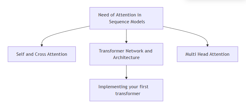
 Self-attention is the core mechanism that allows transformers to process sequential data (like text) by dynamically weighing the importance of different parts of the input.
Self-attention lets each position (e.g., each word in a sentence) look at all other positions and decide which ones to focus on. Unlike RNNs/CNNs, it: processes all positions in parallel (no sequential dependency). Captures long-range dependencies directly (no information decay over distance).
1.This is a great article introducing essential topics in self attention like, positional encoding, query, value ,key ,etc without going deep into the maths.
2.Watch this to get intution of how self attention work
3.This video will help you understand why we need keys, values and query matrices
4.See the coding part in this video to get idea of the working of self attention
Multi-head attention is a powerful extension of self-attention that allows the model to jointly attend to information from different representation subspaces at different positions. Here’s a comprehensive breakdown:
Instead of performing a single attention function, multi-head attention runs multiple parallel attention heads (typically 8-16).Each head learns different attention patterns (e.g., syntactic, semantic, positional relationships). Combines results from all heads to form the final output.
Why it works: Different heads can specialize in different types of relationships (e.g., one head for subject-verb agreement, another for pronoun resolution).
Read this article to get more details
Attention mechanisms have to compute how much focus to place on different parts of the input. It works by:
Comparing a Query (Q) with all Keys (K) using dot products. Scaling the scores by √(dimension of keys) to prevent gradient vanishing. Applying softmax** to get attention weights (0 to 1). Using these weights to compute a weighted sum of Values (V).
The attention function is defined as:
\[\text{Attention}(Q, K, V) = \text{softmax}\left(\frac{QK^T}{\sqrt{d_k}}\right)V\]Where:
The Transformer network is a architecture that relies entirely on self-attention mechanisms to compute representations of its input and output without using sequence-aligned RNNs or convolution. It is the backbone of many modern LLMs like chatGPT(where GPT stands for Generative Pre-trained Transformer),Gemini,Llama, BERT which have been built upon the transformer network Spend the next 2 days understanding the architecture and working of different layers of transformers.
The below link will help you implement a tranformer of your own,this also explains the paper Attention is All You Need Paper which giving the correspoding code.
You can skip topics like Multi-GPU Training,Hardware and Schedule. Feel free to refer to the internet, chatGPT or ask us if you are not able to understand any topic.
This week will give you an in-depth dive into the various types of transformers, and later we’ll begin with LLMs.
| Type | Link |
|---|---|
| Video | Intro to Encoder-Decoder Models |
| Blog | What are Encoder-Decoder Models? |
Transformers are the current state-of-the-art type of model for dealing with sequences. Perhaps the most prominent application of these models is in text processing tasks, and the most prominent of these is machine translation. In fact, transformers and their conceptual progeny have infiltrated just about every benchmark leaderboard in natural language processing (NLP), from question answering to grammar correction.
flowchart TD
  subgraph Inputs [Input Variables]
        direction LR
        Xi[Xi]
        Xj[Xj]
        Xk[Xk]
    end

    Process[???]

    subgraph Outputs [Output Variables]
        direction LR
        yi[yi]
        yj[yj]
    end

    Inputs --> Process --> Outputs
Here the transformer is represented as a black box. An entire sequence of (x’s in the diagram) is parsed simultaneously in feed-forward manner, producing a transformed output tensor. In this diagram the output sequence is more concise than the input sequence. For practical NLP tasks, word order and sentence length may vary substantially.
Here’s a deep dive into the architecture of transformers https://www.exxactcorp.com/blog/Deep-Learning/a-deep-dive-into-the-transformer-architecture-the-development-of-transformer-models
Transformers revolutionized sequence-to-sequence tasks like language translation by using the multi-head attention mechanism instead of recurrent neural networks (RNNs). It processes data in parallel, allowing for more efficient training and handling of long-range dependencies in sequences, overcoming limitations of RNNs.
The encoder-decoder model is a type of neural network that is mainly used for tasks where both the input and output are sequences. This architecture is used when the input and output sequences are not the same length for example translating a sentence from one language to another, summarizing a paragraph, describing an image with a caption or convert speech into text.
It works in two stages:
In an encoder-decoder model both the encoder and decoder are separate networks each one has its own specific task. These networks can be different types such as Recurrent Neural Networks (RNNs), Long Short-Term Memory networks (LSTMs), Gated Recurrent Units (GRUs) or even more advanced models like Transformers as mentioned above.
Encoder-only models use just the encoder part of the Transformer architecture. They are designed to understand the input, but they don’t generate new text. They are great for tasks that need the model to make sense of a sentence or document, like text classification or extracting information.
These models only use the decoder part of the Transformer architecture. They are used for generating text or predicting the next word in a sequence. These models are great for tasks like writing stories or auto-completing sentences.
You can refer to this amazing article talking about encoders and decoders in detail: https://magazine.sebastianraschka.com/p/understanding-encoder-and-decoder
Encoder-only models are commonly used to learn embeddings for classification and understanding tasks. Encoder-decoder models are well-suited for generative tasks where the output strongly depends on the input, such as translation or summarization. Decoder-only models are typically applied to open-ended generative tasks, including question answering and text generation.

Here’s another article about comparing the various tansformer forms https://aiml.com/compare-the-different-transformer-based-model-architectures/
Before we get into optimizations, let’s talk about why traditional Transformers can feel like that one friend who always picks the priciest item on the menu. The problem lies in attention: every word in a sentence has to “pay attention” to every other word to understand context. Sounds fine at first, but for a 1,000-word document that’s 1,000 × 1,000 = 1,000,000 comparisons. Stretch that to 10,000 words, and suddenly you’re looking at 100 million comparisons. Things spiral out of control quickly.
This quadratic growth means both memory use and computation time blow up as documents get longer. It’s like trying to have a group chat where everyone insists on talking to everyone else before saying anything — manageable in a small group, total chaos in a stadium.
That’s where State Space Models (SSMs) come in.
SSMs are a family of models designed to predict how systems evolve over time, traditionally used in control systems engineering. They model sequences with differential equations and have recently been adapted for machine learning tasks.Underpinning SSMs are two simple equations: one describes the internal dynamics of a system that aren’t directly observable, and the other describes how those internal dynamics relate to observable results. That simple, flexible formulation is extremely adaptable for a wide variety of multivariate time series data.
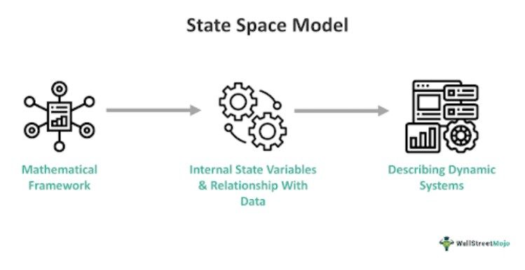
Mamba, a neural network built on a selective variant of structured SSMs, has shown performance on par with Transformers in language modeling.
Go through the articles mentioned below to get an in depth synopsis of SSMs and the optimizations in transformers .
https://huggingface.co/blog/ProCreations/transformers-are-getting-old
https://www.ibm.com/think/topics/state-space-model
| Type | Link |
|---|---|
| Video | Intro to LLMs |
| Blog | What are LLMs? |
| Analysis | Open-source vs Proprietary |
Some private LLMs include ones by Google, OpenAI, Cohere etc. and public ones include the open-source LLMs (lot of which can be found at https://huggingface.co/models).
Deconstruct GPT architecture and implement a minimal LLM
Intuitive explanation of GPT-2: https://jalammar.github.io/illustrated-gpt2/
3D visualisation of inside of LLM: https://bbycroft.net/llm This will offer a unique perspective on how data flows and is processed within the model, enhancing your understanding of its architecture.
A great resource is the video Build Your Own GPT along with the accompanying GitHub repository nanoGPT. This tutorial teaches you how to implement your own LLM from scratch!
Go through this research paper to get a good understanding of BERT. Some more great resources:
Knowledge Distillation: Knowledge Distillation is a pivotal technique in modern Natural Language Processing (NLP) that involves training a smaller “student” model using the outputs of a larger “teacher” model. This process helps in creating models that are more efficient for deployment without significant loss of performance. Below are some essential resources and papers that explore this technique, particularly in the context of BERT and its variations.
More Resources on BERT Variants and Optimizations:
Comparison between BERT, GPT and BART: https://medium.com/@reyhaneh.esmailbeigi/bert-gpt-and-bart-a-short-comparison-5d6a57175fca
Transfer learning is a technique in Natural Language Processing (NLP) where a pre-trained model (already trained on a large dataset) is reused and fine-tuned for a new, specific task instead of training from scratch.
A model (like BERT, GPT, or T5) is first trained on a huge general dataset (e.g., Wikipedia, books, news articles).
It learns general language patterns like grammar, word meanings, and sentence structure.
Instead of training a new model from zero, we take the pre-trained model and adjust (fine-tune) it slightly for a specific task (e.g., spam detection, sentiment analysis, chatbots).
This requires much less data and computing power than training from scratch.
Novice’s LLM Training Guide: https://rentry.org/llm-training provides a comprehensive introduction to LLM Training covering concepts to consider while fine-tuning of LLMs. This is a good starting point to understand what happens “under the hood” during training.
One of the most important component of fine-tuning of LLMs is using quality datasets. This directly affects the quality of the model in the following ways:
Go through the following articles :
Pretraining a GPT-2 model from scratch: https://huggingface.co/learn/nlp-course/chapter7/6?fw=pt Although this is rarely done due to computational costs, but it’ll help you understand the core functionalities.
Keeping up with the latest datasets is crucial for effective fine-tuning. The field of LLM fine-tuning evolves quickly. New instruction datasets appear frequently, and using trending, well-tested ones is crucial. This GitHub repository provides a curated list of trending instruction fine-tuning datasets .
Prompts act like instructions for the model. Effective use of prompt templates can significantly enhance the performance of LLMs. This article from Hugging Face explains how to create and use prompt templates to guide model responses.
Prompt Engineering Guide: https://www.promptingguide.ai/ provides a great list of prompt techniques
Finetuning Llama 2 in Colab demonstrates how large models can be trained on cloud GPUs step by step, even without expensive hardware.
Axolotl : A tool designed to streamline the fine-tuning of various AI models, offering support for multiple configurations and architectures.
Go through the following resource once: Beginners Guide to LLM Finetuning using Axolotl
We’ll discuss two of the PEFT(Parameter-Efficient Fine-Tuning) techniques, where the goal is to fine-tune only a fraction of model parameters instead of the entire model.
LoRA (Low-Rank Adaptation): LoRA reduces the number of trainable parameters by training only a few low-ranked matrices instead of updating all model parameters. This makes fine-tuning efficient, and reduces compute cost. To put in numbers, training a multi-billion parameter model may only require training a few million when using LoRA. Go through this IBM article to learn more about LoRA. Use the following article to implement LoRA: – Implementing LoRA
QLoRA (Quantized LoRA): QLoRA builds on LoRA by combining quantization (reducing precision of weights) with low-rank adaptation. Here, models are stored in lower precision (like 4-bit), and only small LoRA adapters are fine-tuned, making it possible to train large models on a single GPU. Read this article to learn more about QLoRA. Use the following article to implement QLoRA: – Implementing QLoRA
For an in-depth study, here are the research papers presenting LoRA and QLoRA: – LoRA paper – QLoRA paper
Evaluating LLMs is just as important as building them. But this is where the challenge lies – unlike traditional ML Models with clear accuracy metrics, language generation needs specialized evaluation methods to judge fluency and usefulness. Here are a few such methods:
BLEU: BLEU (Bilingual Evaluation Understudy) compares a machine-generated text to one or more human-generated reference texts and assigns a score based on how similar the machine-generated text is to the reference texts. More on BLEU metric and its flaws: https://towardsdatascience.com/evaluating-text-output-in-nlp-bleu-at-your-own-risk-e8609665a213
Perplexity: BLEU evaluates text generation quality against human references, while with Perplexity, we try to evaluate the similarity between the token (probably sentences) distribution generated by the model and the one in the test data. More on Perplexity: https://huggingface.co/docs/transformers/perplexity
ROUGE: ROUGE (Recall-Oriented Understudy for Gisting Evaluation) is another set of metrics used for automatic summarization and machine translation. Unlike BLEU, which focuses on precision, ROUGE is all about recall. It measures the number of n-grams (or word sequences) in the machine-generated summary that also appear in the human-generated reference summaries.
Survey on Evaluation of LLMs: https://arxiv.org/abs/2307.03109 is a very comprehensive research paper on evaluation of LLMs and definitely a recommended read!
Multilingual NLP aims to make AI systems accessible across languages, not just English. The challenge is that the world has 7,000+ languages, many of which are low-resource (little training data). Problems include building translation systems, answering questions across languages, and handling code-switching (when people mix languages in one sentence).
Instead of training a separate model per language, modern approaches use shared multilingual models trained on huge multilingual corpora, allowing transfer learning from high-resource (like English) to low-resource languages.
mBERT, XLM, XLM-R, mT5, NLLB, SeamlessM4T, BLOOMNow we will specifically see what models are used for which tasks:
Problem: How do we automatically translate between languages, especially when parallel datasets (e.g. English ↔ Hindi) are scarce? How it’s solved: Neural MT with sequence-to-sequence transformers trained on large multilingual parallel corpora. Models:
Resources:
Problem: A user asks a question in one language (Hindi), but the answer exists in another language (e.g. in some English Wikipedia). How it’s solved: Multilingual pretrained encoders (like mBERT, XLM-R) can align sentence embeddings across languages, enabling zero-shot transfer. Models:
Resources:
Problem: Searching for “climate change” in Spanish but retrieving English documents. How it’s solved: Use shared multilingual embeddings so queries and documents from different languages map to the same semantic space. Models:
Resources:
Problem: Extract entities (people, places, orgs) in multiple languages with different scripts. How it’s solved: Use multilingual transformer encoders fine-tuned for NER, leveraging character-level embeddings for scripts like Devanagari, Arabic.
Models:
Resources:
Problem: Can we detect emotions or generate summaries across languages? How it’s solved: Fine-tuning multilingual seq2seq models (like mBART, mT5) on sentiment/summarization datasets.
Models:
Resources:
Problem: In many regions (India, Africa), people mix languages: “I like programming, though bugs like me jyda!” How it’s solved: Training multilingual models on code-switched corpora or synthetic data generation.
Models:
Resources:
Some more resources to learn more about Multilingual NLP:
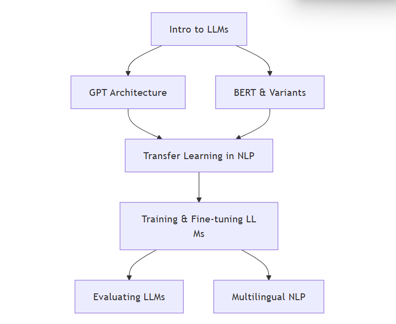
  graph TD
A[Intro to LLMs] --> B[ GPT Architecture]
    A --> C[ BERT & Variants]

    B --> D[ Transfer Learning in NLP]
    C --> D

    D --> E[Training & Fine-tuning LLMs]

    E --> F[ Evaluating LLMs]
    E --> G[ Multilingual NLP]
Brief Intro:
Reinforcement Learning from Human Feedback (RLHF) uses human comparisons to train a reward model that scores candidate text continuations, then applies Proximal Policy Optimization (PPO) to guide an LLM toward safer, more helpful outputs. Reinforcement Learning from AI Feedback (RLAIF) swaps expensive human labels for critiques generated by a stronger model or a rules-based system, enabling faster, cheaper scaling of reward signals.
Key Concepts:
Where It’s Used:
Resources:
Brief Intro:
Group Relative Policy Optimization (GRPO) provides token-level rewards, giving precise control over specific generation behaviors (e.g., math correctness or policy compliance). Efficient RL Fine‑Tuning techniques—such as async rollout architectures and difficulty‑targeted sampling—dramatically reduce compute by focusing on the most informative experiences and keeping GPUs busy.
Key Concepts:
Where It’s Used:
Resources:
Brief Intro: Direct Preference Optimization (DPO) and reward densification explore new approaches for aligning language models more efficiently by using richer feedback and bypassing conventional reward modeling steps. DPO directly optimizes model policy in response to comparison data, often outperforming traditional RLHF in handling ambiguous or multi-objective tasks. Reward densification leverages token-level or intermediate feedback (including from language model critics) to resolve sparse reward issues.
Key Concepts:
Where It’s Used:
Resources:
Brief Intro: Hierarchical RL (HRL) and multi-turn RL techniques allow agents to structure long-term, multi-step reasoning by learning high-level strategies (policies over tasks) and delegating lower-level actions (token or utterance generation). This mirrors human approaches to solving complex problems and offers significant advances for complex dialogue, tool use, and task automation.
Key Concepts:
Where It’s Used:
Resources:
Brief Intro: Multi-agent RL (MARL) extends beyond single-model optimization, focusing on collaboration, negotiation, and emergent strategies between multiple LLMs or agents. Cooperative MARL frameworks allow language agents to solve tasks requiring collective intelligence or simulate realistic social environments for AI development.
Key Concepts:
Where It’s Used:
Resources:
Brief Intro: Recent research shows that reinforcement learning, when scaled and properly designed, can push the reasoning boundaries of LLMs, discovering new cognitive strategies and improving their adaptability. The future points toward hybrid reward sources, verifier-guided optimization, multi-objective alignment, and efficient integration with multimodal tasks.
Key Concepts:
Where It’s Used:
Resources:
The next two weeks covers how NLP extends beyond text to handle speech and multimodal inputs (e.g., combining audio, text, and vision). This week focuses on Text-to-Speech (TTS) — a field that lets machines “speak” like humans, using deep learning to turn written sentences into expressive audio. We’ll learn the pipeline end-to-end and build a working mini-project.
Modern NLP isn’t just about processing text — it’s increasingly about enabling human-like communication across voice, vision, and language. Speech plays a central role in digital assistants, accessibility, and human-computer interaction. This day introduces the importance of speech in AI applications like Siri, Google Assistant, and accessibility tools. We also explore the rise of multimodal systems that integrate multiple input types. Get a quick overview here.
We’ll also reflect on why multimodality matters, especially in a world where humans naturally combine modes when they communicate (e.g., gestures + speech). Tools like Whisper, CLIP, and Flamingo will be briefly mentioned to show how cutting-edge models are moving beyond unimodal processing.
By the end of today, you’ll understand what it means to “go beyond text” and how speech interfaces are becoming central to next-gen NLP systems.
Key Concepts:
Get hands on speech generation here.
TTS converts written input into spoken output. The goal is to produce natural, expressive, and intelligible speech that mimics human speakers of various ages, genders, and emotions. This day focuses on Text Analysis.
E.g., "Dr. Smith won 1st place" → "Doctor Smith won first place"
Grapheme-to-Phoneme (G2P) conversion Text is made up of graphemes (letters), but we speak in phonemes (sounds). This module converts sequences like “ph” into their correct phonetic output (“f”), often using phonetic dictionaries or neural models.
The Text Analysis Module is essentially the “reading comprehension” step for TTS
🔗To get a nice overview : TTS using NLP – Medium 🔗A more detailed pipeline here.
Once the input text is analyzed and converted into linguistic features, the next step is to turn these into a mel-spectrogram—a visual representation of audio over time. This process is handled by the acoustic model, which bridges the gap between text and sound.
Popular neural models like Tacotron (Tacotron uses an attention-based encoder-decoder with RNNs), FastSpeech (FastSpeech and its successor FastSpeech 2 adopt Transformer-based non-autoregressive architecture for fast, parallel spectrogram creation), and VITS (VITS integrates spectrogram generation and waveform synthesis using a variational/adversarial approach for more expressive, end-to-end speech) learn to predict these spectrograms from text sequences by modeling patterns of pitch, duration, and intensity.
These spectrograms serve as intermediate representations that capture the acoustic characteristics of speech, ready to be transformed into waveforms by a vocoder in the next stage.
Now we learn how vocoders like WaveNet or HiFi-GAN generate audio waveforms from spectrograms.
Once the mel-spectrogram is generated from input text, we need to convert this visual-like representation of sound into an actual audible waveform — that is, the raw audio you can hear. A waveform is simply a series of pressure values over time that simulate sound waves. Traditional vocoders used signal processing techniques to approximate these waves, but they often sounded robotic or unnatural.
Neural vocoders solve this by using deep learning to model the complex relationships between spectrogram features and natural audio waveforms. These models are trained on large datasets of paired spectrograms and real human speech, learning how to generate high-fidelity audio one sample at a time.
For example, WaveNet uses autoregressive generation (predicting one sample at a time based on previous ones), while HiFi-GAN uses non-autoregressive methods to produce audio much faster, making it suitable for real-time applications. Different vocoder architectures (WaveNet, WaveGlow, HiFi-GAN) trade off between speed, quality, and complexity.
See detail about HiFi-Gan here See benchmarking framework comparing vocoder performance and trade‑offs (quality, latency, generalization) across multiple models in a unified setup.
We now explore how modern TTS systems are evolving beyond just “reading text aloud.” Recent research focuses on making speech more expressive, personalized, inclusive, and efficient — especially for deployment on edge devices like smartphones or IoT hardware.
Cutting-edge systems now synthesize speech that reflects emotion, adapts to new speakers with minimal data, and handles multilingual or code-switched inputs — all while keeping latency low enough for real-time interaction.
Expressive and Emotional TTS Models now capture subtle emotions like joy, sadness, urgency, or sarcasm — crucial for human–AI interaction in assistants, games, or therapy bots. See more. → Example: Emotional Tacotron, GPT-SoVITS
Personalized and Adaptive Voices TTS can adapt to new speakers from just seconds of reference audio, enabling personal voice clones, celebrity voices, or synthetic dubs. → Popular methods: Few-shot speaker adaptation, zero-shot voice cloning
Multilingual + Code-Switched TTS Seamless voice synthesis across multiple languages and dialects, even when mixed mid-sentence (code-switching), is especially relevant for India, Southeast Asia, and Africa. See more. → Models like NLLB-TTS, SeamlessM4T, and Festival-Multilingual
Real-time Edge Deployment Efficient neural vocoders (like HiFi-GAN and LPCNet) allow TTS on low-powered devices without a GPU, unlocking accessibility for mobile and embedded applications.
Adaptation to low-resource settings is a growing research frontier. This includes building TTS systems for underrepresented languages, dialects, or speaker groups where data is sparse.
Zero-shot / Few-shot Voice Cloning: Generate high-quality speech from a new speaker using just a few seconds of audio (or no audio at all, with metadata). See more on this paper.
TTS for Low-Resource Languages: Techniques like multilingual pretraining, transfer learning, and synthetic data augmentation help build systems even for languages with few recordings. A good PDF here.
Speaker Adaptation: Personalize TTS to user voice, accent, or speaking style with minimal training time and resources.
This article, discusses Speech Recognition and its application of it by implementing a Speech to Text and Text to Speech Model with Python.Analytics Vidhya Guide Article on recent trends here.
In these two days, you’ll put everything you’ve learned into practice by building your own TTS system using pretrained models. This hands-on project will give you a better understanding of how the components of a TTS system—text processing, spectrogram generation, and vocoding—come together to produce human-like speech.
Goal: Understand the end-to-end pipeline, experiment with inputs, and visualize outputs.
Resources:
This week explores how machines convert spoken language into written text using Automatic Speech Recognition (ASR) systems and how modern AI models fuse speech, text, and visual inputs to build more intelligent, human-like agents. We’ll cover key models like Whisper, wav2vec, and GPT-4o, and dive into practical applications such as transcription, voice-controlled assistants, and multimodal chatbots.
You’ll gain both theoretical and hands-on understanding of:
Today, we begin exploring Automatic Speech Recognition (ASR) —the technology that converts spoken language into text. ASR powers everything from virtual assistants like Siri and Alexa to automated subtitles on YouTube and real-time transcription services. Understanding the basic workflow of ASR helps set the stage for upcoming days.
ASR involves capturing speech, preprocessing the audio, extracting features, and finally decoding it into text using language and acoustic models. It’s not just about recognition—challenges like background noise, speaker variability, accents, and domain-specific vocabularies make ASR a rich and evolving research area.
Modern ASR has shifted from traditional modular systems (acoustic + language + pronunciation models) to End-to-End Deep Learning approaches that simplify the pipeline while improving performance.These End-to-End ASR systems directly map audio to text using architectures like CTC (Connectionist Temporal Classification), Attention-based Seq2Seq, and RNN-T, leveraging powerful deep learning methods like CNNs, RNNs, and Transformers.
To further improve performance—especially in multilingual or low-resource settings—modern ASR systems use self-supervised learning (e.g., wav2vec 2.0) or massive multitask pretraining (e.g., Whisper). These models learn from raw audio at scale and can be fine-tuned for specific languages or domains.
See a nice course on ASR here.
In these two days we explore modern ASR systems that work across multiple languages, noise levels, and accents.
Whisper is a multilingual, multitask ASR model trained on over 680,000 hours of multilingual and multitask supervised data collected from the web. It uses an encoder-decoder Transformer architecture similar to those used in machine translation. Its design makes it highly effective for:
Under the hood, Whisper converts raw audio into a log-mel spectrogram, which is fed to a Transformer encoder. The decoder then autoregressively generates the transcribed text.
You can experiment with different Whisper model sizes (tiny, base, small, medium, large) and observe trade-offs in speed and accuracy.
Multilingual speech data you can use to test or fine-tune models
wav2vec 2.0 is a self-supervised model by Meta AI. Instead of relying on labeled data, it learns powerful speech representations directly from raw audio. It’s pre-trained using contrastive loss, where the model distinguishes real future audio segments from fake ones.
After pretraining, wav2vec 2.0 can be fine-tuned on a relatively small labeled dataset for transcription. This makes it especially valuable in low-resource or code-switched speech settings.
wav2vec 2.0 has a convolutional encoder that processes raw waveform and a Transformer for context modeling. The final output is optimized using Connectionist Temporal Classification (CTC) loss or, in some versions, attention-based decoders.
Fine-tuning for Audio Classification with Transformers
Modern ASR models have evolved beyond traditional HMM-GMM pipelines into fully neural architectures. Common components include:
Automatic speech recognition using advanced deep learning approaches: A survey
Today, we consolidate our understanding of deep learning architectures used in ASR and compare the performance, trade-offs, and design choices across prominent systems like Whisper, wav2vec 2.0, and DeepSpeech.
Modern ASR has moved from traditional HMM-GMM based systems to powerful end-to-end neural architectures. These approaches unify the acoustic, pronunciation, and language models into a single trainable pipeline.
Automatic Speech Recognition using Advanced Deep Learning Approaches
Overview of end-to-end speech recognition
Automatic speech recognition using advanced deep learning approaches: A survey
A book on ASR by Deep learning approach Automatic Speech Recognition :A Deep Learning Approach
We now compare three leading deep learning-based ASR models—each with different trade-offs in latency, architecture, and accuracy.
| Model | Architecture | Inference Style | Strengths | Weaknesses |
|---|---|---|---|---|
| DeepSpeech | RNN + CTC | Offline | Simpler architecture, open-source | Less accurate, not multilingual |
| wav2vec 2.0 | Transformer + CTC | Offline/Fast | Self-supervised, high accuracy | Needs language-specific tuning |
| Whisper | Encoder-Decoder (RNN-T) | Offline | Multilingual, robust to noise, translation support | Slower inference, heavy compute |
At each time step, the model selects the token with the highest probability. It’s the simplest and fastest method, but it doesn’t consider the overall sequence, which can lead to suboptimal results.
Instead of picking just the top token, beam search keeps track of the top k most likely sequences (beam width). This allows the model to explore better combinations of words, significantly improving transcription quality—especially in longer or ambiguous utterances.
External language models (like n-gram or Transformers) can be combined with ASR outputs to refine decoding. The LM helps ensure the generated text is syntactically and semantically plausible, especially in noisy or low-resource scenarios.
| Use Case | Preferred Model | Reason |
|---|---|---|
| Real-time captioning | wav2vec (small) | Faster decoding |
| Batch transcription | Whisper / wav2vec | High accuracy |
| Noisy environments | Whisper | Trained on noisy data |
Now we will explore the evolution of multimodal systems that unify speech, text, and images to enable more natural and intelligent AI applications.
Modern AI models are increasingly multimodal — meaning they can understand and generate across multiple input types. For example, systems can now answer questions about an image using spoken queries or perform visual search via voice commands. This is possible thanks to advancements in cross-modal architectures and retrieval-augmented generation (RAG), where information is retrieved from external sources and fused with model outputs.
Cross-modal RAG (Retrieval-Augmented Generation) Traditional RAG systems retrieve relevant text snippets from a knowledge base to help generate better textual responses. In cross-modal RAG, the retrieval and generation steps span across different modalities. For example, a model may retrieve textual data in response to an audio query, or retrieve relevant images or audio clips based on a text prompt. This enables more natural and flexible interactions — such as asking a question via speech and receiving a multimodal answer that includes both a spoken response and a visual reference.
A github repo on multimodal RAG here. An Easy Introduction to Multimodal Retrieval-Augmented Generation for Video and Audio by Nvidia.
Audio-to-text QA This involves asking questions through spoken language and receiving textual answers. It combines automatic speech recognition (ASR) with question answering (QA) systems. The ASR first transcribes the speech input, then the QA model identifies and returns the appropriate answer. This is useful in hands-free environments or accessibility-focused tools.
WavRAG: Audio-Integrated Retrieval Augmented Generation for Spoken Dialogue Models
Voice-command visual search This is the situation where users issue voice commands to search through visual datasets (images, videos, documents). For example, a system might support queries like “show me photos with red cars taken at night” or “find the slide where Einstein is mentioned.” This requires integrating speech recognition, semantic understanding, and image retrieval in a unified pipeline. Modern systems use models like CLIP or GPT-4o to map both voice inputs and images into a common representation space, enabling effective cross-modal search.
Dive into the architectures and systems enabling multimodal learning. These models leverage shared embeddings or transformer blocks that process diverse modalities together (e.g., text and images).
Topics:
Apply what you’ve learned by building either a robust ASR system or an entry-level cross-modal agent. This project allows you to integrate speech, text, and possibly vision into a functioning application.
Project Options:
NLP is wide , so hold tight to your coffee mugs and until then..
Contributors