Roadmap to Computer Vision 🦝

Welcome to the Computer Vision Roadmap by Programming Club IITK, wherein we’ll be building right from the preliminary techniques of Image Processing and thereafter largely cover the intersection of Machine Learning and Image Processing. Thereafter, we shall be touching upon various cutting-edge techniques in GenAI and Representational Learning (specifically, GNNs) which are mildly related to the domain of CV and CNNs. We’re expecting that you’re here after completing the Machine Learning Roadmap, which covers the basics of Machine Learning, Neural Networks, Pipelines and other preliminary concepts; so in this roadmap, we assume that the explorer has that knowledge and we pick up from there. Even if you have explored Machine Learning independently, we strongly recommend you to go through the ML Roadmap once before starting this. Although all topics are not prerequisite, but most of them are.

Also do remember, in case you face any issues, the coordies and secies \@Pclub are happy to help. But a thorough research amongst the resources provided before asking your queries is expected :)

🦝 Meta-Knowledge

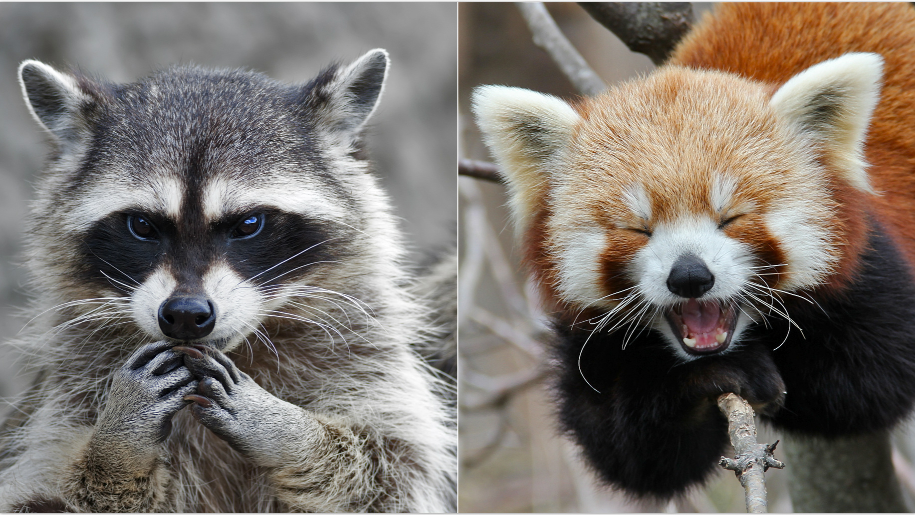
We started off our Machine Learning journey with the example of automating the differentiation process between a Raccoon 🦝 and a Red Panda. In the ML Roadmap we played a lot with numbers and datasets, but how do we convert the images of a Raccoon into forms which can be interpreted by our models? More importantly, how are these images represented by computers? Can we simply run the model on these images or do we require to alter the image in order to get good results? Let’s try to find the answers of these questions.

Manipulation of the mathematical representation of Digital Images in order to extract, alter, add or remove some form of information is Image Processing. When we perform some image processing algorithm/method on an image, we get image. For instance, enhancing image quality, converting a colored image to black and white image, or applying any Instagram filter counts as image processing.

meta-kn
Digital Image Representation

Then what is Compute Vision? CV is a field of artificial intelligence (AI) that uses machine learning and neural networks to teach computers and systems to derive meaningful information from digital images, videos and other visual inputs—and to make recommendations or take actions when they see defects or issues. Image processing may not always utilize AI/ML, while on the other hand, CV is strictly a subset of AI. This Article by IBM provides a great introduction to CV. You can go through the following material to understand the difference between CV and Image Processing better:

Optional Read: What is CV and Understanding Human Vision

🦝 Meta-Roadmap

This section largely focusses on how to use this roadmap in a efficient manner, and how you can play around with the same. Note that most of the Computer Vision courses or learning materials focus mostly on the Convolutional Neural Net (A special type of NN which we shall explore later) part of CV, which is an extremely small subset of what Image Processing and CV truly encompasses. It is also not very intuitive and does not help one in understanding the logic behind how object identification or classification is happening (You’d be able to classify an image as a Raccoon 🦝 or a Red Panda, but you’d not know WHAT the CNN is actually doing behind the scenes; it’s essentially a Blackbox).

In this roadmap, we start off with low level Image Processing which involves understanding the theory of Digital Images and their manipulation without the use of these backboxes and cover the same in the first two weeks. This shall hopefully provide you a decent intuition behind how things might work behind the scenes and the “logic” behind the processing. Post that, we bring Deep Learning into the picture in week 3 by introducing CNNs. The first 3 weeks MUST be followed in the prescribed order.

Post CNNs, we delve deep into the famous CNN architectures and use cases in weeks 4 and 5. You can study these two weeks in any order because they are largely independent. Note that in both the weeks, we start off by providing the non-ML approach to solving the problem at hand which builds your logic and then move on to how these problems can be solved using CNNs.

Henceforth, you can take three paths:

Continue with the applications of Detection and Segmentation in Week 6, explore Face Detection and Recognition, Pose Estimation, Motion and Tracking.
Switch to learning Generative Models. For this track, you can skip week 6 and directly do weeks 7 through 10; and then 12
Explore a unique type of Neural Networks called Graph Neural Networks in week 11.

These three tracks are largely independent of each other so can be explored in any order.

🦝 Recurring Resources

Throughout the Roadmap, we’ll be constantly referring to a few course websites and lecture notes. So it’s recommended that you keep referring them and exploring the stuff we’ve not included if it seems interesting. It’s highly recommended to read this section thoroughly and keep these resources handy/at the back of your mind while you’re on this CV Journey.

CS131 Computer Vision: Foundations and Applications: This is an introductory Computer Vision course which covers fundamental methods to process, manipulate and extract information from images. This largely covers mathematics, transformations and non-ML algorithms. I shall refer this intensively in the first 2 weeks, and then later during recognition, detection and segmentation sections. Following are some important links:
OpenCV Course: This is an instructive hands on course on OpenCV which consists of a series of notebooks which guide you through how to implement various Computer Vision and Image Processing methods via OpenCV library of Python. This GitHub Repository consists of all the resources of the course. This course is divided into two parts: - OpenCV: Starts off by introducing how digital images and color spaces work and goes on to explain various transformation, filters and methods like Convolutions, Thresholding, Moments etc. Then it has notebooks which cover practical applications like detection, recognition, tracking, style transfer etc. - Deep Learning CV: As the name suggests, this section provides a hands on learning approach to Deep Learning using PyTorch, Keras and TensorFlow. This also contains various projects which shall help you to apply this knowledge to real life.

👾How to use this Course? Mastering Machine Learning requires a mastery of theory, mathematics and applications. Unfortunately this course only fulfills the application part of it and does not include theory and mathematics. As we proceed through this roadmap, we’ll provide you various resources to master the theory and mathematics of various methods. Use this course in tandem with the theory provided in order to have an all round understanding. Keep referring to these notebooks everyday and going through the topics as and when they are covered in the week.
OpenCV Official Tutorials: The Tutorial articles on the official site of OpenCV provide a decent introduction to theory, but most importantly provide a great walkthrough of the OpenCV library, which is really important for implementing any CV project in Python. You can find the tutorials via the following link: https://docs.opencv.org/4.x/d6/d00/tutorial_py_root.html
Computer Vision: Algorithms and Applications Book by Richard Szeliski: This book covers almost all the topics required to have a great foundational knowledge of Image Processing, but might be a bit too advanced and extensive at times if followed along with the resources provided. You can give it a read for some, or all topics if you find learning better this way. Here’s a link to downloading the book for free: https://szeliski.org/Book/
Introduction to Computer Vision Course by Hany Farid, Prof at UC Berkeley: This playlist consists of concise (mostly less than 10 mins) videos which brilliantly capture the mathematics, logic and visualization of various introductory CV and Image Processing concepts, along with their implementation in python. The course is so easy to follow that if you’re not able to understand any concept via the resources provided, it’s guaranteed that a video from this playlist will help you understand it. You can find the playlist here: https://www.youtube.com/playlist?list=PLhwIOYE-ldwL6h-peJADfNm8bbO3GlKEy
CS231n: Deep Learning for Computer Vision: This builds on CS131 by introducing CNNs, their training, architectures, Deep Gen Models and other methods. This course shall be referred week 3 onwards. Following are some important links:
CS224W: Machine Learning with Graphs: Provides an introduction to Graphs, and Graph Neural Networks. Will be constantly referred in week 11.
CS236: Deep Generative Models: Gold Standard Gen AI course. Shall be referred constantly from weeks 8 through 10.
CS294-158-SP20: Deep Unsupervised Learning:
- Course Website
CSE 599: Generative Models:
- Course Website
Jeremy Jordan Website: This Website maintained by Jeremy Jordan has a bunch of interesting articles on various Machine Learning and Data Science topics, along with guided resources and lecture notes of various famous courses. Although this website will not be repeatedly referred, you can go through the content if you find it interesting.

Considering we are done and dusted with the prelude, let’s get started with the Computer Vision Journey 👾

🦝 Table of Contents

🦝 Week 1: Image Processing I

You might want to constantly refer to the Exercises of the first chapter of CV by Szeliski, provide an intensive practice of all almost all the concepts that we shall cover in the first 2 weeks. You might want to practice simultaneously or at the end; completely upon you.

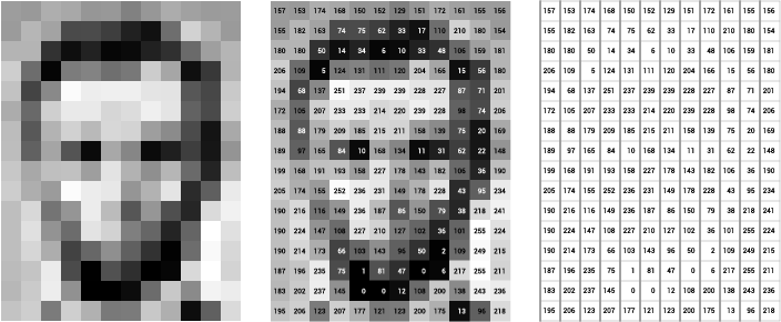
👾Day 1: Digital Images and Linear Algebra Review

In digital world an image is a multi-dimensional array of numeric values. It is represented through rows & columns each storing data in numeric format which represents a particular region of Image. The individual cell is called pixel, the image’s dimension is represented through number of pixels in it’s height & width. To learn in detail, [click here](http://lapi.fi-p.unam.mx/wp-content/uploads/1.4-Opt_ContinousImages.pdf.

Linear Algebra will be extremely important in implementing various transformations. For a refresher, refer to the following PDFs:

👾Day 2: Color and Color Spaces

col-space
Color Space Comparison

Color is a vital element in computer vision and digital imaging, influencing how we perceive and interpret visual information. In the world of programming and image processing, color spaces play a crucial role in manipulating and analyzing images. Understanding color spaces is essential for anyone working with image data, as they provide different ways to represent and process color information.

A color space is a specific organization of colors, allowing us to define, create, and visualize color in a standardized way. Different color spaces are used for various applications, each offering unique advantages depending on the context. The most common color spaces include RGB (Red, Green, Blue), HSV (Hue, Saturation, Value), HSL(Hue, Saturation & Lightness) and CMYK(Cyan, Magenta, Yellow, and Key).

Read more about Color Space, here & more here

👾Day 3: Pixels, Filters and Convolutions

Refer to the lecture notes of fourth lecture of CS131 for today’s topics.

🐼Image Histograms

Main Resource: Image Processing from Szeliski

An image histogram is a type of histogram that acts as a graphical representation of the tonal distribution in a digital image. It plots the number of pixels for each tonal value. By looking at the histogram for a specific image a viewer will be able to judge the entire tonal distribution at a glance. Go through the following resources for understanding Histograms better:

🐼Image Filters

Filters are simply functions (linear systems) applied on an image which output a new image. The new pixel values are some linear transformations of the original pixel values. Filters are used to extract important information from the image.

Following video will provide an intuitive understanding of Filters: How do Image Filters work

Main Resource to understand Image Filters: Linear Filtering and Neighborhood Operators by Szeliski

filters
Image with various filters applied

🐼 Convolutions

Convolutions are a fundamental operation in the field of image processing and computer vision, forming the backbone of many advanced techniques and algorithms. They are essential for extracting features from images, enabling us to detect edges, textures, and patterns that are crucial for understanding and analyzing visual data.

At its core, a convolution is a mathematical operation that combines two functions to produce a third function, expressing how the shape of one is modified by the other. In the context of image processing, this involves overlaying a small matrix called a kernel or filter on an image and performing element-wise multiplication and summation. The result is a new image that highlights specific features based on the chosen kernel.

convolutions

Watch this amazing video on convolutions

Convolutions are extensively used in various applications, including:

Edge Detection: Identifying boundaries and contours within images. Blurring and Smoothing: Reducing noise and enhancing important features. Sharpening: Enhancing details and making features more distinct. Feature Extraction: In neural networks, convolutions help in identifying and learning important features from images for tasks like classification and object detection.

Understanding convolutions is critical for anyone working with image data, as they provide the tools to transform raw images into meaningful information. In this section, we will delve into the principles of convolutions, explore different types of kernels, and demonstrate how they are applied in practical image processing tasks. By mastering convolutions, you’ll gain the ability to manipulate and analyze images with precision and efficiency.

Watch the the first three videos to understand Convolutions in Depth.

👾Day 4: OpenCV 101

OpenCV is a library designed to offer a common infrastructure for computer vision applications and to accelerate the use of machine perception in commercial products. Its primary goal is to provide a ready-to-use, flexible, and efficient computer vision framework that developers can easily integrate into their applications.

You can download OpenCV using pip. Refer here for some Video demonstration. This is a blog on OpenCV.

Moreover, as and when you keep covering concepts, refer to the relevant notebooks of the OpenCV course provided in Recurring Resources Section to understand implementation of that concept via OpenCV

Until now we’ve covered Color Spaces, Digital Images, filters and convolutions. Go through the following tutorials to implement methods relating to these topics in OpenCV:

👾Day 5: Thresholding

Thresholding is one of the segmentation techniques that generates a binary image (a binary image is one whose pixels have only two values – 0 and 1 and thus requires only one bit to store pixel intensity) from a given grayscale image by separating it into two regions based on a threshold value. Hence pixels having intensity values greater than the said threshold will be treated as white or 1 in the output image and the others will be black or 0. Go through the following articles to understand thresholding:

Refer to notebook 9 of OpenCV Course for practical demonstration.

Thresholding

👾Day 6: Morphological Transformations and Edge Detection

🐼 Binary Image Processing

While non-linear filters are often used to enhance grayscale and color images, they are also used extensively to process binary images. The most common binary image operations are called morphological operations, because they change the shape of the underlying binary objects. Some of the well known Morphological Transformations are: Opening, Closing, Dilation, Erosion, Majority.

To get an in depth understanding of Morphological Transformations, go through the following extract from Szeliski: Binary Image Processing

For implementation of binary processing methods, go through the following article: Morphological Transformations in OpenCV

Morphological transformations

🐼 Edge Detection

Edge detection and line detection are techniques in computer vision that play a crucial role in various applications, such as image processing, object recognition, and autonomous systems. The principle behind edge detection involves identifying areas of significant intensity variation or gradients in the image. Edges often correspond to changes in color, texture, or intensity, and detecting them is crucial for tasks like object recognition, image segmentation, and feature extraction.

Canny Edge Detection

Main Theory Resource: Notes of Lecture 5 and Lecture 6 of CS131.

For Diving Deep into Edge Detection, go through the following links:

👾Day 7: Fourier Transforms and Contours

🐼Fourier Transforms

The Fourier Transform is an important image processing tool which is used to decompose an image into its sine and cosine components. The output of the transformation represents the image in the Fourier or frequency domain, while the input image is the spatial domain equivalent. In the Fourier domain image, each point represents a particular frequency contained in the spatial domain image.

Go through the following resources for an in depth understanding and implementation of Fourier Transforms:

🐼 Contours

Contours can be explained simply as a curve joining all the continuous points (along the boundary), having same color or intensity. The contours are a useful tool for shape analysis and object detection and recognition. These are largely used in detection and matching applications. For a better understanding, refer to notebook 11 of OpenCV Tutorial and follow the link:

OpenCV Contours Tutorials

🦝 Week 2: Image Processing II

👾Day 1: Key points, Image Features, Feature Descriptors

🐼 Keypoints

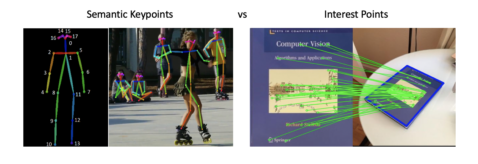
Semantic Keypoints and Keypoint Matching

Keypoints are the same thing as interest points. They are spatial locations, or points in the image that define what is interesting or what stand out in the image. Interest point detection is actually a subset of blob detection, which aims to find interesting regions or spatial areas in an image. The reason why keypoints are special is because no matter how the image changes… whether the image rotates, shrinks/expands, is translated (all of these would be an affine transformation by the way…) or is subject to distortion (i.e. a projective transformation or homography), you should be able to find the same keypoints in this modified image when comparing with the original image.

Keypoints are extremely important in Computer Vision and the detection of keypoints has various applications for instance, -time face matching, object tracking, image contouring, image stitching, motion tracking etc. To have a better understanding of keypoints, refer to this medium article and this stackoverflow discussion

🐼 Image Registration

Let’s say you have two images of the same cute Raccoon 🦝, but the orientation of raccoon in each image is different? A human brain can easily understand which point corresponds (or “aligns”) to which point of the Raccoon in both the images. But how do we attain this with Computer Vision? The answer is Image Registration.

Image registration is the process of spatially aligning two or more image datasets of the same scene taken at different times, from different viewpoints, and/or by different sensors. This adjustment is required in multiple applications, such as image fusion, stereo vision, object tracking, and medical image analysis. Go through the following article to have a better understanding of Image Registration: https://viso.ai/computer-vision/image-registration/#:~:text=Image%20registration%20algorithms%20transform%20a,tracking%2C%20and%20medical%20image%20analysis.

🐼 Robust feature matching through RANSAC

RANSAC (and variants) is an algorithm used to robustly fit to the matched keypoints to a mathematical model of the transformation (“warp”) from one image to the other, for example, a homography. The keyword here is “robustly”: the algorithm tries really hard to identify a large (ideally, the largest) set of matching keypoints that are acceptable, in the sense they agree with each other on supporting a particular value of the model. For a better understanding of RANSAC, go through the following content:

MIT Lecture Slides
CS131 Lecture 7 Notes: These also cover some important concepts on Keypoint Localization and Invariant Keypoints. Go through these topics as they are important for the next subsection.

🐼 Scale Invariant Keypoint Detection

Let’s say you have a video of a Raccoon 🦝 going beautifully through trash 🗑️, and you need to track the motion of the same. These applications require keypoint detections across a wide number of similar images at vastly different scales without the prior knowledge of the size of the Raccoon. For such forms of keypoint detection, we need a function which takes in the image, and irrespective of the scale of the image returns the same keypoints. These are done via various functions and methods like Average Intensity, Difference of Gaussians and Harris-Laplacian. To understand these algorithms, go through CS131 lecture 8 notes

🐼 Scale Invariant Feature Transform (SIFT) Algorithm

SIFT Algorithm flowchart

By extracting distinctive features from images, SIFT allows machines to match those features to new images of the same object. Using SIFT, you shall be able to recognize the Cute Raccoon 🦝 from any angle and orientation, even after distortions and blurring. SIFT follows a four-step procedure:

Constructing a Scale Space: To make sure that features are scale-independent
Keypoint Localisation: Identifying the suitable features or keypoints
Orientation Assignment: Ensure the keypoints are rotation invariant
Keypoint Descriptor: Assign a unique fingerprint to each keypoint

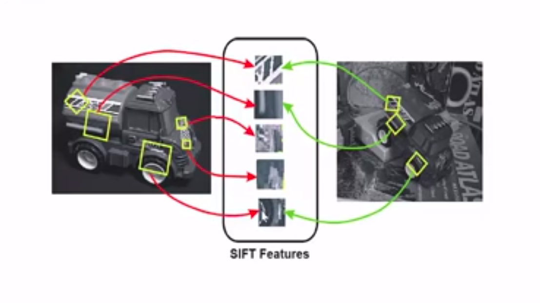
Feature mapping using SIFT

Go through CS131 lecture 8 notes, along with the following blogs in order to understand the mathematics and implementation of SIFT:

🐼 Histogram of Oriented Gradients (HOG)

Histogram of Oriented Gradients

We’ve already talked enough about Histograms and Gradients, so understanding this algorithm should not really be tough. The histogram of oriented gradients (HOG) is a feature descriptor used in computer vision and image processing for the purpose of object detection. The technique counts occurrences of gradient orientation in localized portions of an image. Go through CS131 lecture 8 notes and these blogs to learn HOG:

👾Day 2: Pyramids and Wavelets

(Day 2 shall be pretty heavy, but the next 2 days are extremely light so according to convenience you can prolly spend a bit more time with Pyramids and Wavelets and speed-run the next 2 days. )

Main Study Resource: Pyramids and Wavelets from Szeliski

Changing the scale of image (reducing and increasing it size) is so fundamental that we simply don’t try to question the intricacies and algorithms behind it and take it for granted. Today we shall largely talk about up-sampling and down-sampling images and how can pyramids and wavelets be utilized in image processing.

🐼Pyramids

Image Pyramid

Working with images with lower resolution is extremely memory, time and power efficient because we have less amount of information (to be specific, signals) to process. A common way to do this is via a combination of blurring and down-sampling; and these processes can be implemented iteratively to form a pyramid-like scheme. This method is called the method of pyramids and on the basis of the types of filter we’re using for blurring, we can have different types of pyramids. Take a look at the following videos to get a better understanding:

Gaussian Pyramid: Largely used for display resolution, dimensionality reduction, efficient search and match etc.
Laplacian Pyramid: For sub-band analysis, de-noising, compression

Go through this NPTEL video for a better understanding of applications of Pyramids.

Refer to the first 4 subsections of Pyramids and Wavelets from Szeliski to understand more about Interpolation (up-sampling from lower to higher resolution), Decimation (down-sampling from higher to lower resolution) and Multi-Resolution Representations.

Here is an OpenCV tutorial on how to implement Image Pyramids

🐼Sub-Band Coding

In signal processing, sub-band coding (SBC) is any form of transform coding that breaks a signal into a number of different frequency bands, typically by using a fast Fourier transform, and encodes each one independently. This decomposition is often the first step in data compression for audio and video signals.

Imagine you have a really long book on Raccoons 🦝 that you need to summarize. Instead of summarizing the whole book in one go, you might find it easier to break the book into chapters and summarize each chapter individually, for instance divide the book into subtopics like their inherent laziness, their trash-picking skills, cuteness (subjective, but I strongly agree), attempted scary faces etc. Sub-band coding works on a similar principle for signals (like audio or images).

The idea is to:

Improve Efficiency: By breaking down a signal into smaller frequency bands, you can process and compress each part more efficiently.
Reduce Redundancy: Different parts of a signal might contain redundant information. Sub-band coding helps to identify and remove this redundancy.
Enhance Quality: When you process each sub-band separately, you can apply techniques that are best suited for each band, leading to better overall quality.

Sub-Band Coding is primarily used in Audio Compression, Image Compression, Speech Processing and Telecommunications. We shall majorly look at the Image Compression part of it in this section.

Go through the following video to understand Sub-Band Coding better: https://www.youtube.com/watch?v=bci7xMFVnvs

🐼Wavelets and Multi-Resolution Processing

Wavelets are a famous alternative to Pyramids, and are filters that localize a signal in both space and frequency (like the Gabor filter) and are defined over a hierarchy of scales. Wavelets provide a smooth way to decompose a signal into frequency components without blocking and are closely related to pyramids.

The fundamental difference between Pyramids and Wavelets is that traditional pyramids are overcomplete, i.e., they use more pixels than the original image to represent the decomposition, whereas wavelets provide a tight frame, i.e., they keep the size of the decomposition the same as the image.

Go through the remaining portions of Pyramids and Wavelets from Szeliski to understand how Wavelets are constructed and their applications in image blending.

👾Day 3: Resizing Algorithms

In the last section, we primarily talked about simply down-sampling and up-sampling wherein we were just scaling the length and width of the image by a factor. The issue with that is that this might lead to artifacts or loss of important features and information. For this, we use Seam Carving Algorithms to efficiently resize the image from $(m*n)$ to $(m’ * n’)$ pixels.

Human vision is more sensitive to edges, because they show a high Image Gradients, so it is important to preserve edges. But even if we remove contents from smoother areas, we’ll likely retain information. We utilize a gradient-based energy function for this kind of transformation, which detects the importance of various regions by calculating sum of absolute values of the x and y gradients.

We’ve identified which pixels are ‘important’ and which are ‘less important’. How do we remove the ‘unimportant pixels’ in a way which preserves the core information of the image. For this, we define a ‘Seam’, that is a connected path of pixels from top to bottom or left to right which minimizes the energy function.

The concept of Gradient-based Energy Function and Seam is used to reduce the size of the image, via Seam Carving Algorithm.

A similar approach can be employed to increase the size of images by expanding the least important areas of the image.

Go through CS131 Lecture 9 Notes (download the file if it does not render inline) to understand these concepts better and explore its implementation via code.

👾Day 4: Strides and Padding

Let’s take a detour from the status quo and learn some basic concepts in image processing which shall be helpful in building up to Convolutional Neural Networks.

In the realm of image processing and neural networks, strides and padding are two crucial concepts that significantly impact the behavior and output of convolutional operations. Understanding these concepts is essential for effectively designing and implementing convolutional neural networks (CNNs) and other image processing algorithms.

Strides Strides determine how the convolutional filter moves across the input image. In simpler terms, strides specify the number of pixels by which the filter shifts at each step. The stride length affects the dimensions of the output feature map.

Stride of 1: The filter moves one pixel at a time. This results in a detailed and often larger output. Stride of 2: The filter moves two pixels at a time, effectively down-sampling the input image. This produces a smaller output but reduces computational complexity. Choosing the right stride is important for balancing detail and efficiency. Smaller strides capture more detailed information, while larger strides reduce the size of the output, which can be beneficial for computational efficiency and reducing overfitting in deep learning models.

Padding Padding refers to the addition of extra pixels around the border of the input image before applying the convolutional filter. Padding is used to control the spatial dimensions of the output feature map and to preserve information at the edges of the input image.

Valid Padding (No Padding): No extra pixels are added. The output feature map is smaller than the input image because the filter cannot go beyond the boundaries. Same Padding (Zero Padding): Extra pixels (usually zeros) are added around the border to ensure that the output feature map has the same spatial dimensions as the input image. This allows the filter to cover all regions of the input image, including the edges. Padding helps to maintain the spatial resolution of the input image and is crucial for deep neural networks where preserving the size of feature maps is often desirable.

Why Strides and Padding Matter Control Over Output Size: By adjusting strides and padding, you can control the size of the output feature maps, which is crucial for designing deep neural networks with specific architectural requirements. Edge Information Preservation: Padding helps to preserve edge information, which is important for accurately capturing features located at the boundaries of the input image. Computational Efficiency: Strides can be used to down-sample the input image, reducing the computational burden and memory usage in deep learning models.

Here’s video for above concepts. Refer videos 4-5.

Here’s an amazing blog, make sure to check it out.

👾Day 5: Geometric Transformations and Geometry Detection

🐼 Geometric Transformations

Earlier this week, we explored as to how up-scaling, down-scaling and resizing is performed on images via various transformations. Another set of important operations are the geometric transformations like translations, skewing, rotations, projections etc, which are essentially linear transforms. Ideally, you’d think that matrix multiplication should work in such a case, right? But the problem is that underlying pixels of a screen can’t be transformed into other shapes, and they will remain squares of fixed sizes. So we need to create certain mappings such that we are able to perform these transformations, while preserving the structure of the fundamental blocks of an image: the square pixels.

This is a good time to revise key-points, feature descriptors, pyramids and wavelets because these concepts shall be constantly used in building up geometric transformations.

🐯Warping

Warping a Raccoon Image

Geometric Image Transformations are also called Warping. There are largely 2 ways to warp an image:

Forward Mapping: In this method, each pixel in the source image is mapped to an appropriate place in the destination image. Thus, some pixels in the destination image may not be mapped. We need interpolation to determine these pixel values. This mapping was used in our point-morphing algorithm.
Reverse Mapping: This method goes through each pixel in the destination image and samples an appropriate source image pixel. Thus, all destination image pixels are mapped to some source image pixel. This mapping has been used in the Beier/Neely line-morphing method.

Following are some good resources to understand basic warping:

Post gaining this basic intuition of Warping, go through the following resources for understanding the development of modern warping techniques, and Feature-based morphing which is an application of Geometric Transformation:

🐼 Contour Matching

Main Resource: Notebook 12 of OpenCV Course

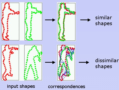
Contour Matching

An important application of image processing is detecting and recognizing objects. Feature mapping is a relatively complex concept, and using it to differentiate between a square and triangle is like using the Quadratic Formula to solve $x^2 - 1 = 0$ 👾. There are methods via which we can differentiate between objects, and detect them without detecting key-points and mapping them.

🐯 Hu Moments

Image moments are a simply the weighted average of image pixel intensities. These weighted averages can be evaluated via various formulae. If we are able to define a unique moment for a shape, which is translation, scale, and rotation invariant, we will have a metric which can uniquely identify a shape. Hu Moment is such a moment that is translation, scale, and rotation invariant. TO learn more about moments and shape matching using hu moments:

🐯Contour Detection and Matching

We explored contours last week, now we shall use contours to match shapes. Note that a contour can define the boundary of a shape, helping in eliminating all the features which are irrelevant in shape identification and matching. To learn about the same, follow this TDS blog

🐼 Line, Circle and Blob Detection

Main Resource: Notebook 13 of OpenCV Course

In Edge Detection, we explored the Hough Transform. Note that edge detection is fundamental to any kind of shape detection because the boundaries of shapes are comprised of edges. In this section, we shall be using Hough Transform for Line, Circle and Blob detection. Go through the following resources for the same:

[Blob Detection Theory](https://repo.ijiert.org/index.php/ijiert/article/download/565/539/1086
Blob Detection via DOG, DOH, Connected Components
Hough Circle Transform OpenCV Tut
Line, Circle, Blob Detection using Hough
Detecting Ellipses in Images

🐼 Finding the Raccoon 🦝🥺

Main Resource: Notebook 14 of OpenCV Course

Find the Raccoon

The Cute Raccoon 🦝 is lost in an image full of hundreds of animals, and you’re missing the Raccoon🥺. For finding it, we need to spot the cute raccoon from this image wherein there are multiple animals. The raccoon is just hidden amidst all the noise and distraction, and MUST be spotted. Note, that mathematically speaking, the raccoon is nothing but a visual pattern 🤖 which can be easily spotted if we have it’s isolated image. We can just check as to which region in the larger image matches the pattern of the raccoon. This procedure in Image Processing is called Template Matching. For understanding how to find the Raccoon, go through the following links:

👾Day 6 and 7: Practice and Hand-on Stuff

Exercises of the first chapter of CV by Szeliski provide an intensive practice of all almost all the concepts covered in the last 2 weeks. You needn’t complete all the questions, you can selectively pick.

Along with these questions, you can try out all or some of these hands on projects (Don’t use CNNs or pre-trained models; the first 2 weeks were all about non black-box based image processing techniques implemented from scratch):

🐼 Face Detection and Recognition

Description: Implement a system that can detect faces in real-time from a webcam feed and recognize known individuals.

Key Concepts:

Haar Cascades or HOG + Linear SVM for face detection.
LBPH, Eigenfaces, or Fisherfaces for face recognition.

Project Steps:

Capture video from a webcam.
Detect faces in each frame.
Recognize detected faces.
Display names or IDs of recognized faces on the video feed.

🐼 Edge Detection and Image Filtering

Description: Develop an application that applies different image filters and edge detection algorithms to an input image.

Key Concepts:

Sobel, Canny, and Laplacian filters for edge detection.
Gaussian, median, and bilateral filters for smoothing and noise reduction.

Project Steps:

Load an image from the disk.
Apply various edge detection algorithms.
Implement different image filtering techniques.
Display the original and processed images side by side.

🐼 Barcode and QR Code Scanner

Description: Develop an application that can scan and decode barcodes and QR codes in real-time.

Key Concepts:

Image thresholding and binarization.
Contour detection and perspective transformation.
Barcode and QR code decoding using libraries like zbar or OpenCV.

Project Steps:

Capture video from a webcam.
Detect and localize barcodes or QR codes in each frame.
Decode the detected codes.
Display the decoded information on the video feed.

🦝 Week 3: Convolutional Neural Networks

Third week onwards, we shall primarily focus on application of Deep Learning in the domain of Image Processing and Computer Vision, wherein we’ll start out with the basic CNN architecture and build our way to Generative Models

In Image Processing, we learnt about Convolution Operations, and in the ML Roadmap we explored Feedforward neural networks. It’s not tough to guess that CNNs will somehow integrate the Convolution Operation into Feedforward Neural Networks. How does this happen? Why does this work? Why not flatten the image into a vector? We shall answer these questions this week and also practically implement a basic CNN architecture.

👾Day 1: Intro to CNNs for Visual Recognition

Before we start off with theory, I’d highly recommend you to binge the following videos as they will provide you a great insight into the the workings of CNN (+the visualizations are hot, so these will help build strong intuition and visual understanding):

🐼What are CNNs?

Convolutional Neural Networks (CNNs) are a class of deep neural networks commonly used for analyzing visual data. They are particularly effective for tasks involving image recognition, classification, and processing due to their ability to capture spatial hierarchies and patterns within images. Developed in the late 1980s, CNNs have since revolutionized the field of computer vision and have become the cornerstone of many modern AI applications. Unlike traditional neural networks, which treat input data as a flat array, CNNs preserve the spatial structure of the data by using a grid-like topology.

ConvNet

🐼Key Components of CNNs

Convolutional Layers: These layers apply convolution operations to the input, using learnable filters to detect various features such as edges, textures, and patterns. Each filter slides over the input image, producing a feature map that highlights the presence of specific features.
Pooling Layers: Pooling layers reduce the spatial dimensions of feature maps, helping to down-sample the data and make the network more computationally efficient. Common pooling operations include max pooling and average pooling.
Fully Connected Layers: After a series of convolutional and pooling layers, the high-level reasoning in the network is done via fully connected layers. These layers flatten the input data and pass it through one or more dense layers to perform classification or regression tasks.
Activation Functions: Non-linear activation functions like ReLU (Rectified Linear Unit) introduce non-linearity into the model, allowing it to learn complex patterns. Activation functions are applied after convolutional and fully connected layers.
Regularization Techniques: Techniques like dropout and batch normalization are used to prevent overfitting and improve the generalization capability of the network.

🐼Convolutional Layers

Convolutional layers are the fundamental building blocks of Convolutional Neural Networks (CNNs), which are designed to process and analyze visual data. These layers play a crucial role in detecting and learning various features within images, such as edges, textures, and patterns, enabling CNNs to excel in tasks like image classification, object detection, and segmentation.

A convolutional layer performs a mathematical operation called convolution. This operation involves sliding a small matrix, known as a filter or kernel, over the input image to produce a feature map. Each filter detects a specific feature, such as a vertical edge or a texture pattern, by performing element-wise multiplication and summing the results as it moves across the image.

Watch videos 6-8 for understanding Convolutional Layers

You can read the below blog, to get further on CNNs. Introduction to CNN (Read Here).

Go through the second lecture of CS231n which gives an overview of Image Classification Pipelines. You can find the lecture slides here

👾Day 2: Refresher: Loss Functions, Optimization and BackProp

We’ll devote the second day primarily to revise concepts we’ve already covered in the ML roadmap and bring them into context with respect to CNNs by introducing SoftMax. Go through the following videos and lecture slides (you can also skim through the content if you feel you remember it):

Lecture 3 of CS231n and its Lecture Slides
Lecture 4 of CS231n and its Lecture Slides

👾Day 3: Pooling, FC Layers, Activation Functions

Today, we shall learn about certain CNN-specific concepts and patch them together to understand the architecture of a general CNN.

🐼 Pooling Layers

Unlike convolutional layers having kernels with trainable parameters, in pooling there’s no sort of trainable params. So if they aren’t trainable, what’s it’s use, basically pooling layers are used to compress/reduce the size of data while still having retained it’s important aspects.

There are various kinds of Pooling Layers- Max Pooling, Min Pooling, Average Pooling, etc. Here’s a short blog on Pooling Layers. If you are interested in some depths, check out this

Watch video 9.

🐼 Fully Connected Layers

After Convolutional & Pooling layers, let’s move to Fully Connected Layers. An FC layer is a Dense Neural Network Layer, which leads to a Numerical Output, achieving our task of utilizing image data for tasks like classification, object detection, etc. A fully connected layer refers to a neural network in which each neuron applies a linear transformation to the input vector through a weights matrix. As a result, all possible connections layer-to-layer are present, meaning every input of the input vector influences every output of the output vector.

🐼 Activation Functions

We’ve already explored various activation functions in the Machine Learning Roadmap. To learn about some activation functions specific to CNNs and also revise the earlier ones, follow this link
Here’s a blog on Sigmoid & SoftMax Activation functions Here’s a research paper highlighting importance of an Activation function.

🐼 Connecting the Dots: The CNN Architecture

Go through the Fifth Lecture of CS231n and its Lecture Slides to understand how Convolutional Layers, Pooling Layers, Fully Connected Layers and Activation Functions are utilized to construct a CNN.

Here’s a great visualization explaining how to chose kernel size while building a CNN.

👾Day 4: Data Preprocessing, Regularization, Batch Norm, HyperTuning

🐼 Data Preprocessing

As learnt earlier, the images provided in the dataset might not be fit to pass through the model due to varying sizes, varying orientation of objects, noisy images, blurry image, incomplete image etc. Moreover, sometimes certain models perform better on filtered images or images in different color spaces which calls for a need to highly preprocess images before running them through the model. Methods like histogram normalization, greyscale filters, resizing, cropping, opening, closing, dilation are extremely helpful in the preprocessing step.

For understanding more about the preprocessing step, refer the first section of Lecture 6 of CS231n and its lecture slides

🐼 Regularization

As you delve deeper into Convolutional Neural Networks (CNNs), you’ll encounter challenges like overfitting and the need for more efficient and effective model architectures. Regularization techniques are essential tools to address these challenges, enhancing the performance and generalization capabilities of your CNN models.

Regularization techniques are strategies used to prevent overfitting, where a model performs well on training data but poorly on unseen data. These techniques introduce constraints and modifications to the training process, encouraging the model to learn more general patterns rather than memorizing the training data.

Dropout:

Dropout is a technique where, during each training iteration, a random subset of neurons is “dropped out” or deactivated. This prevents neurons from co-adapting too much and forces the network to learn redundant representations, making it more robust. Typically, dropout is applied to fully connected layers, but it can also be used in convolutional layers.

Batch Normalization:

Batch normalization normalizes the output of a previous activation layer by subtracting the batch mean and dividing by the batch standard deviation. This stabilizes and accelerates the training process, allowing for higher learning rates. It also acts as a regularizer, reducing the need for dropout in some cases.

Read this blog to grasp on above topics.

In depth implementation of Batch Normalization, along with a review of HyperTuning for CNN has been covered in the second section of Lecture 6 of CS231n and its lecture slides

👾Day 5: Data Augmentation, Optimizers Review

🐼 Data Augmentation

Image Augmentation

Sometimes, the dataset you have is not large enough, or does not capture all variations of the images leading to a pathetic accuracy score. For improving the training dataset, you can augment it by applying random transformations and filters to the same, helping in expanding the dataset and making it diverse at the same time.

Read this article to get idea of image augmentation: https://towardsdatascience.com/image-augmentation-14a0aafd0498

How to do data augmentation using tensorflow : https://colab.research.google.com/github/tensorflow/docs/blob/master/site/en/tutorials/images/data_augmentation.ipynb

No need to mug up the commands, rather learn about what possible data augmentation you can do with TensorFlow.

🐼 Optimizers Review and Second-Order Optimization

Gradient Descent, it’s variants and the optimizations on it (NAG, RMSProp, ADAM etc) utilize First-Order optimization as they only involve evaluation of first-order derivative of the loss function. Methods like the Newton Method and Quazi-Newton Methods utilize Second-Order Optimization, providing better results sometimes, but at the cost of space and time cost.

For a review of topics studied so far, their implementation, reviewing Optimizers studied in ML Roadmap and exploring Second Order Optimization, go through the Seventh Lecture of CS231n and its lecture slides

👾Day 6: Deep Learning Hardware and Frameworks

🐼CPU v/s GPU

A CPU has Fewer cores, but each core is much faster and much more capable; great at sequential tasks
A GPU has significantly higher number of cores, but each core is much slower and “dumber”, making it ideal for parallel tasks

Deep Learning is simply a large number of Linear Transformations (and a few non-linear as well), and a major reason for high compute is not the compute required for a single, or a sequence of operations, but the sheer scale of the number of independent operations performed. In order to tackle this, we can parallelize the independent tasks, and assign less compute to individual processes rather than allocating a huge compute on a single process or a sequence of dependent processes. This makes training DL models on GPU much more efficient.

🐼Computational Graphs DL Frameworks

The most relevant DL Framework now a days are Tensorflow and PyTorch. Caffe, which is a framework by Facebook is largely outdated and not used.

For learning more about DL Hardware, Tensorflow and PyTorch, go through the 8th lecture of CS231n and its lecture slides

Refer to these notes for an overview of the DL Hardware and Frameworks

This concludes the theoretical part of Introduction to Convolutional Neural Networks.

👾Day 7: Hands on Stuff

It’s time to get hands on some Practical Implementations.

Your task is to create a model for “Automatic Covid disease detection by Chest X-ray Images through CNN model”.

Description: You are given a dataset of X-rays images. Dataset is divided into train and test data further divided into three categories - Normal , Covid and Viral Pneumonia. You need to create a common directory for train and test images (hint: you need to import os library for this, look on internet for working) then resize the images and normalize data if needed, Split train data into train data and validation data. Convert categorical data into numerical data. You can also use ImageDataGenerator function from Tensorflow Library. Then Build a CNN model and fit the model on train data, validate the model and play with the hyperparameters for eg. no of layers, no. of filters, size of filters, padding, stride. You can also try different optimizers and activation functions. Also plot the your results for eg, loss vs epochs , accuracy vs epochs for train and validation data. You are expected to use Google Colab for this task.

DATASET: Here’s Dataset.

🦝 Week 4: Segmentation and CNN Architectures

👾Day 1: Segmentation and Clustering

Main Resource for the day: Notes of Lecture 10 of CS131. Constantly refer them while covering the subtopics.

🐼 Segmentation

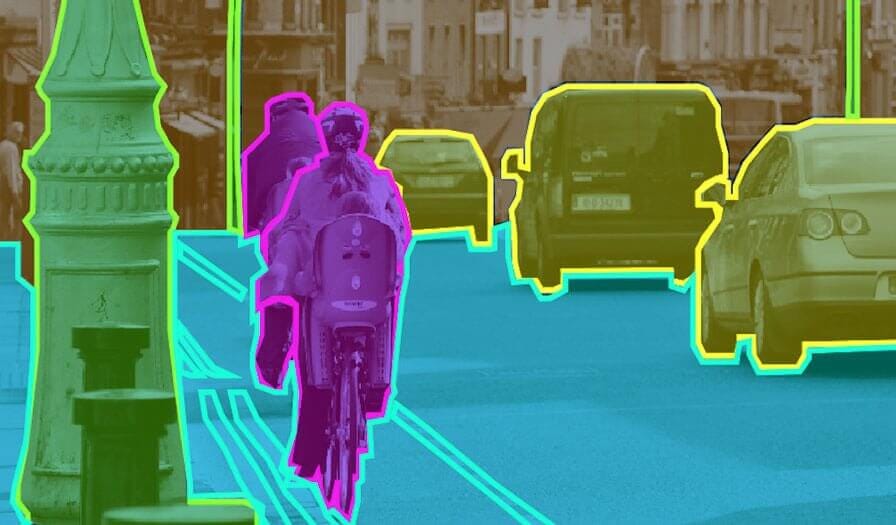
Image Segmentation

Image segmentation refers to the task of dividing an image into segments where each pixel in the image is mapped to an object. This task has multiple variants such as instance segmentation, panoptic segmentation and semantic segmentation. In simpler terms Image segmentation looks at an image and assigns each pixel an object class(such as background, trees, human, cat etc.). This finds several use cases such as image editing, background removal, autonomous driving and whatnot. it differs from object detection as this technique creates a mask over the object rather than a bounding box.
It is majorly divided into 3 types:

Semantic Segmentation
Instance Segmentation
Panoptic Segmentation

Go through this article for a refresher on Image Feature Extraction, as they will be helpful in the following weeks.

Go through the following articles to understand Segmentation better:

Intro to Image Segmentation
Applications and Types of Image Segmentation
Image Segmentation and its Types
Image Segmentation Techniques
Intersection over Union metric for segmentation evaluation
🐼 Clustering

We’ve already covered most of the Clustering algorithms in Machine Learning Roadmap. Here, we shall explore how clustering is used in image processing and CV.

Image Segmentation is the process of partitioning an image into multiple regions based on the characteristics of the pixels in the original image. Clustering is a technique to group similar entities and label them. Thus, for image segmentation using clustering, we can cluster similar pixels using a clustering algorithm and group a particular cluster pixel as a single segment.

Go through the following articles for understanding the role of clustering in image segmentation:

🐼Mean Shift for Segmentation

Main resource for the subtopic: First Section of Notes of Lecture 11 of CS131

Mean shift is a mode-seeking clustering algorithm widely used for the purposes of segmentation and searching for regions of interest in an image. This technique involves iteratively moving data points towards regions of maximum density, using a search window and a kernel. The aim is to determine both the extent of the search and the way in which the points are moved. The density of points is evaluated in a region around a point defined by the search window. For a better understanding, go through the following videos:

👾Day 2: Types of Segmentation

Today, we shall explore various types of segmentations in depth:

🐼Semantic Segmentation

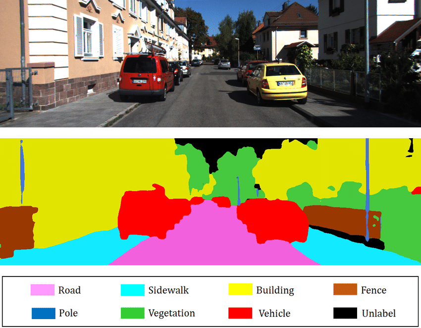
Semantic Segmentation

Semantic segmentation tasks help machines distinguish the different object classes and background regions in an image.

For understanding the concept and theory, refer to this article by IBM
For understanding CNN architecture for Semantic Segmentation, refer to this blog by Jeremy Jordan.
Famous Semantic Segmentation Techniques and their implementation
Paper on Fully Convolutional Networks for Semantic Segmentation: This website contains the original research paper, as well as various GitHub Repositories with implemented code.

🐼 Instance Segmentation

Instance Segmentation

Instance segmentation, which is a subset of the larger field of image segmentation, provides more detailed and sophisticated output than conventional object detection algorithms. It predicts the exact pixel-wise boundaries of each individual object instance in an image. More on instance segmentations:

Introduction to instance segmentation
Difference between instance and semantic segmentation
Instance Segmentation Algorithms
Paper on Mask R-CNN for Object Instance Segmentation: Also contains github repos containing implementations of the papers

🐼 Panoptic Segmentation

Types of Segmentation

Panoptic Segmentation is a computer vision task that combines semantic segmentation and instance segmentation to provide a comprehensive understanding of the scene. The goal of panoptic segmentation is to segment the image into semantically meaningful parts or regions, while also detecting and distinguishing individual instances of objects within those regions. In a given image, every pixel is assigned a semantic label, and pixels belonging to “things” classes (countable objects with instances, like cars and people) are assigned unique instance IDs. More on Panoptic Segmentation:

👾Day 3: Transfer Learning

🐼 What is Transfer Learning

Transfer learning is a machine learning technique where a model trained on one task is reused or adapted as the starting point for a model on a different but related task.
It leverages knowledge gained from the source task to improve learning on the target task, especially when labeled data for the target task is limited.
Benefits include reduced training time and the ability to achieve better performance on the target task with less data.
Common in applications like natural language processing, computer vision, and speech recognition.
Techniques include fine-tuning existing models, feature extraction, and domain adaptation.

An exercise which will teach you how to use transfer learning in your projects using TensorFlow.

🐼 General Resources for CNN Architectures

In the next few days, we’ll try to understand various CNN Architectures, their evolution and applications. Some of the general resources which cover the same are given below:

CS231n Lecture 9 and its Lecture Notes (Don’t get baffled by the number of pages lmao 🦝, most of the slides contain images and flowcharts)
ConvNet Lecture Notes
CNN Architecture Notes by Aman

You don’t need to cover these resources this week 👾, these are just reference materials for the next few weeks.

👾Day 4: LeNet-5 and AlexNet

Before starting, watch this video to understand the architectures of ConvNets and their evolutions.

🐼 LeNet-5

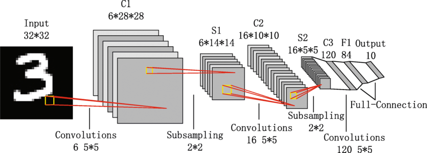
LeNet-5 Architecture

The LeNet-5 Architecture was the very first ConvNet Architecture to be developed and implemented. It’s salient features are:

Every convolutional layer includes three parts: convolution, pooling, and nonlinear activation functions
Using convolution to extract spatial features (Convolution was called receptive fields originally)
The average pooling layer is used for subsampling.
‘tanh’ is used as the activation function
Using Multi-Layered Perceptron or Fully Connected Layers as the last classifier
The sparse connection between layers reduces the complexity of computation

For understanding the model better, take a look at this and this article.

Try to read and implement this research paper on Document Recognition via LeNet.

🐼 AlexNet

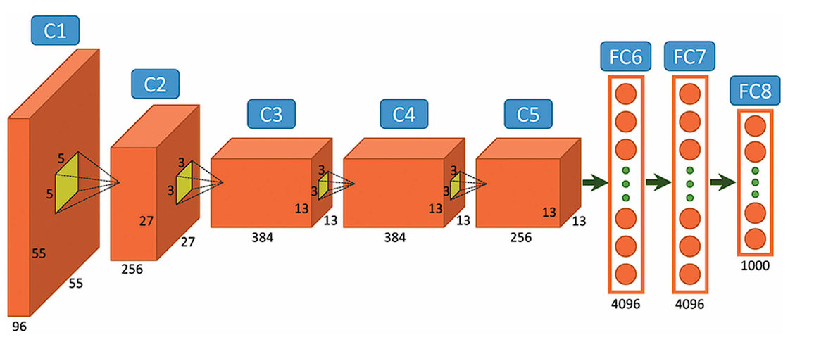
AlexNet Architecture

AlexNet was one of the first models to leverage the computational power of GPUs extensively. The model was trained on two GPUs, which allowed for faster training times and handling of large datasets like ImageNet. This network was very similar to LeNet-5 but was deeper with 8 layers, with more filters, stacked convolutional layers, max pooling, dropout, data augmentation, ReLU and SGD.

Read this article on AlexNet

The article also contains code implementation of AlexNet, Brownie Points for understanding and implementing it.

👾Day 5: ZFNet

The architecture is a refined version of AlexNet, focusing on improving performance by adjusting hyperparameters and exploring the learned features in greater depth.
ZFNet retained basic architecture of AlexNet but made some architectural adjustments,particularly in the first few layers.
AlexNet used 11x11,5x5 and 3x3 filter sizes while ZFNet used 7x7 filter size in the first layer only and 3x3 in the latter layers only. This reduced the training compute.
There is stride of 4 in the first layer of AlexNet while in ZFNet there is stride of 2 used.
AlexNet used Local Response Normalization while ZFNet used Local Contrast Normalization
Utilizes a Deconvolutional Network to visualize the learned features and understand the workings of convolutional layers.

Read this article on ZFNet to see how it improves and builds upon AlexNet.

👾Day 6: VGG16, VGG19 and GoogleNet

🐼 VGG16 and VGG19

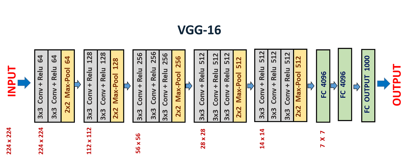
VGG16 Architecture

VGG16 and VGG19 were introduced by the Visual Geometry Group (VGG) at Oxford University.
These architectures were presented in the paper Very Deep Convolutional Networks for Large-Scale Image Recognition and stood out in the ILSVRC 2014.
VGG16 and VGG19 are known for their simplicity and depth, consisting of 16 and 19 layers, respectively thus giving their names.
It was recognized by Oxford Researchers that the operation performed by a $55$ kernel is same as the operation performed by 2 $33$ kernels with a pooling layer in the middle. So rather than increasing the kernel size, they only used $3*3$ kernels, but increased the depth of the model. This significantly increased the accuracy of the model.

For understanding the VGNet Architectures, go through this article

Post completing VGNet, go through this GFG Blog which summarizes and compares all the ConvNet Architectures studied to far.

👾Day 7: U-Net

U-Net Architecture

The architecture is named U-Net because of its U-shaped structure, consisting of an encoder (down-sampling path) and a decoder (up-sampling path).
U-Net has a symmetric architecture with an encoder (contracting path) and a decoder (expanding path). This allows it to effectively capture and utilize both local and global contextual information.
Read this article on UNET Architecture to get a deeper understanding.
Follow this article and implement image segmentation using UNet by yourself.
Paper on U-Net implementation for Biomedical Image Segmentation: This site contains a research paper on U-Net Implementation along with the github repositories with code implementation. Try to go through the paper and understand its implementation

🦝Week 5: Object Recognition and Detection

In the previous week, we learnt about Segmentation and its various types. This is a good time to introduce you to the large categories of applications of Computer Vision and the differences between them. CV has primarily 4 applications: Detection, Recognition, Segmentation and Generation.

Object recognition is simply the technique of identifying the object present in images and videos. In Image classification, the model takes an image as an input and outputs the classification label of that image with some metric (probability, loss, accuracy, etc). Object detection aims to locate objects in digital images. Image segmentation is a further extension of object detection in which we mark the presence of an object through pixel-wise masks generated for each object in the image.

To understand the differences better, go though the following articles:

👾Day 1: Object Recognition

An object recognition system finds objects in the real world from an image of the world, using object models which are known a priori. This task is surprisingly difficult. Humans perform object recognition effortlessly and instantaneously. You’d be able to recognize a cute raccoon 🦝 instantaneously without any efforts, but for a computer to learn it and then recognize it is a largely complex task.

Recognizing a Cute Raccoon

First, it is important to understand Object Recognition Model pipelines and system design, for it involves various complex processes like Feature Detection, Hypothesis formation, Modelbase and Hypothesis verification. We’ve already studied the Feature Detection process, and how does the hypothesis function look like for a general CV task. In this week, we shall explore specific hypothesis for Object Recognition and Classification. For a foundational understanding of the pipelines and hypothesis, go through the following Chapter: https://cse.usf.edu/~r1k/MachineVisionBook/MachineVision.files/MachineVision_Chapter15.pdf)

Image Recognition Pipeline

We’ve learnt about K Nearest Neighbor Algorithm and how we can use it for segmentation. Note that KNN is a versatile algorithm for classification, and hence can be used in object recognition as well. To understand its implementation in Object Recognition use case and the problems with it, go through Notes of Lecture 11 of CS131

👾Day 2: Object Detection by Parts

🐼 Introduction to Object Detection

Object detection is a technique that uses neural networks to localize and classify objects in images. This computer vision task has a wide range of applications, from medical imaging to self-driving cars. As opposed to detection, recognition also involves localization and involves construction of bounding boxes around specific objects, and detection of multiple image classes from same image.

For a basic introduction to Image Detection, go through the following articles:

🐼 Object Detection by Parts

Previously, we learnt about methods for detecting objects in an image; in this section, we shall learn about methods that detect and localize generic objects in images from various categories such as cars and people.

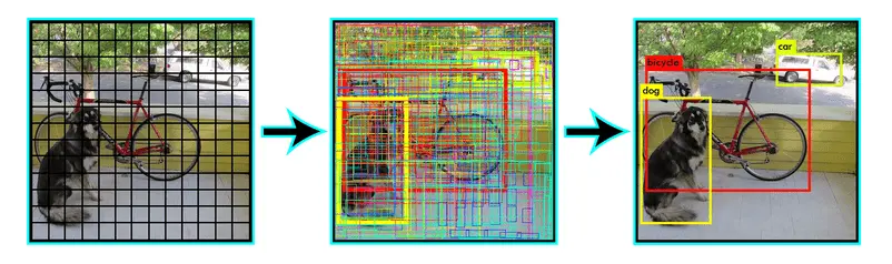
Note, that Object Detection is very similar to Classification and Recognition in the sense that mostly any Detection problem can be converted into a classification problem by adding additional steps like Image Pyramid, Sliding Window and Non-Maxima Supression.

Go through the notes of Lecture 15 and Lecture 16 of CS131 for this topic.

🐯 SlidingWindow Detector

Sliding Window Pipeline

In object detection problems, we generally have to find all the possible objects in the image like all the cars in the image, all the pedestrians in the image, all the bikes in the image, etc. To achieve this, we use an algorithm known as Sliding window detection.

Let’s say we wish to recognize all the cute raccoons 🦝 from an image of a forest. A sliding window is a fixed-size rectangle that slides from left-to-right and top-to-bottom within an image. We will pass a sliding window through the image of the forest, and at each stop of the window, we would:

Extract the ROI
Pass it through our image classifier
Obtain the output predictions

For understanding how this works in detail and how to implement Sliding Window, go through:

🐯 Dalal and Triggs

Dalak and Triggs suggested using Histograms of Oriented Gradients, along with Support Vector Machines for the purposes of Image Detection, specifically Human Detection and Face Recognition. You can find the original paper here. For a visual understanding, go through the following videos:

🐯 Deformable Parts Model (DPM)

The simple sliding window detector is not robust to small changes in shape (such as a face where the eyebrows are raised or the eyes are further apart, or cars where the wheel’s may be farther apart or the car may be longer) so we want a new detection model that can handle these situations.

Go through notes of Lecture 15 of CS131.
Simultaneously watch the following short videos: DPM intro, DPM for rigid bodies, DOM results

You can then optionally go through Lecture 16 of CS131, which provides modern trends, methods for improving accuracy etc.

👾Day 3: InceptionNet and ResNets

Refer to the relevant parts of the following resources for GoogleNet (InceptionNet) and ResNets:

CS231n Lecture 9 and its Lecture Notes (Don’t get baffled by the number of pages lmao 🦝, most of the slides contain images and flowcharts)
ConvNet Lecture Notes
CNN Architecture Notes by Aman
🐼 InceptionNet

InceptionNet Architecture Logic

IneptionNet ,developed by google, achieved a huge milestone in CNN classifiers when previous models tried to improve the performance and accuracy by just adding more and more layers. The Inception network, on the other hand, is heavily engineered. It uses a lot of tricks to push performance, both in terms of speed and accuracy.

its most notable feature is the inception modules that it uses. These modules are an arrangement of 1x1,3x3,5x5 convolution and max-pooling layers that aim to capture features on different ‘levels’. These levels refer to the different sizes an object can be in an image

Read this article to learn more about the inception net and its different versions.

🐼 ResNets

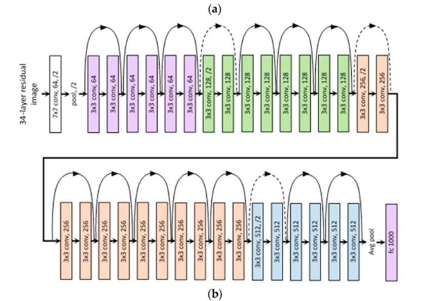
ResNet Architecture

ResNet or Residual Networks is similar to Inception Net in a sense because both aimed to solve the problem of CNN using more and more layers to try to get better efficiency. This architecture uses the residual blocks that work in a similar way to RNNs. They add a weighted part of the input to the output of the convolutional layer in order to mitigate the loss of information. Given below is an image of a residual block.

Read this article to learn more about residual networks.

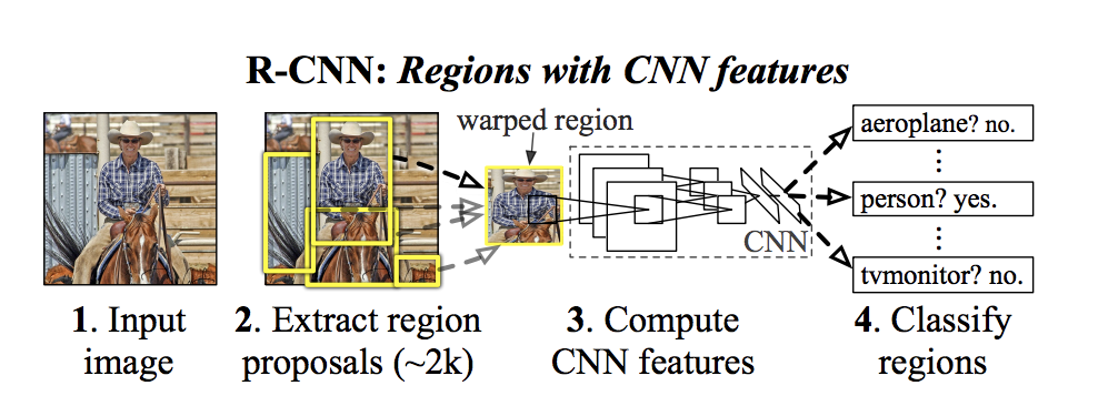
👾Day 4: Region-Based CNN, Fast RCNN, Faster RCNN

R-CNN Procedure

Go through 11th Lecture of CS231n and its lecture notes for a refresher on Detection and Segmentation, and a detailed explanation of R-CNN and its optimized versions.

Region-Based-CNN(R-CNN),introduced in 2013, was one of the first successful methods for object detection using CNNs. It used multiple networks to propose regions with possible objects and then passed these regions thrugh other networks to produce confidence scores.But there was a problem with this model, it was slow ,as it fed each proposed region(read the given article for more information) individually through the CNN.

Improving upon this, came the Fast R-CNN in 2015,it solved some of the problems by eliminating the need to pass multiple regions, it rather passed the whole image.

Finally the Faster-RCNN was proposed to improve the Fast-RCNN .It did so by changing the method it used to search the probable regions. It was around 20 times faster than the original R-CNN.

🔎 Read this article to review your understanding about R-CNN, Fast R-CNN, Faster R-CNN and YOLO(discussed later).

👾Day 5: RoboFlow and YOLO

🐼 RoboFlow

Roboflow is one of the most useful platforms when it comes to computer vision. It provides you with basically everything essential for computer vision and more ranging from Data Management, Model Training, Deployment and Collaboration.

Data Management - Roboflow facilitates data annotation, preprocessing, and organization, including tasks like image labeling (bounding boxes, segmentation), dataset management, and version control.
Model Training - Users can train custom computer vision models or utilize pre-trained models for tasks such as object detection and image classification. It supports popular frameworks like TensorFlow and PyTorch.
Deployment - The platform enables easy deployment of trained models across various environments, including mobile devices, web applications, and edge devices. Tools are available for optimizing model size and latency.
Collaboration - Teams can collaborate effectively on projects through role-based access control and version control for datasets and models.

To get a more comprehensive idea of what roboflow can do take a look at this video and follow it through for a quick implementation of a project.(for a more interesting approach, try to make a project of your own with a custom dataset)
Also check out this official blog and this playlist by RoboFlow themselves.

Roboflow can be used to implement YOLO, one of the most useful models around in the domain of computer vision. Let us learn more about it.

🐼 YOLO

YOLO

YOLO (stands for You-Only-Look-Once), is a series of computer vision models that can preform object detection, image classification, and segmentation tasks. I would say that YOLO is a jack of all trades in computer vision. YOLO has seen constant development over the years starting with the first YOLO model YOLOv1 to the current latest YOLOv10. It is a single shot algorithm that looks at the image once and predicts the classes and bounding boxes in a single forward pass, this makes YOLO much faster than other object detection models. This single stage architecture also aids in the training process making it more efficient than others

Here’s a simplified breakdown of how it works. Image is divided into a grid and split into cells. Each cell predicts bounding boxes for objects it might contain and then features are extracted. Each cell analyzes the image features within its area using CNNs. These features capture the image’s details. Bounding boxes and confidence scores are predicted. Based on the extracted features, the model predicts-bounding box coordinates(if multiple overlapping bounding boxes are predicted for the same class then yolo performs NMS to eliminate bounding boxes) and confidence score.

Non-Maxima Suppression (NMS): If multiple cells predict bounding boxes for the same object, NMS selects the most confident one and discards overlapping or low-confidence boxes. Here is a video to get an idea about NMS

🔎 Read this article to review your understanding about R-CNN, Fast R-CNN, Faster R-CNN and YOLO.

👾Day 6: Hands on YOLO

Go through this article from machinelearningmastery for an overview of whatever we’ve studied this week and a list of important RCNN and YOLO papers, and Code projects which you can implement.

For a comparative analysis of Image Detection algorithms available at present, go through this article

🔎 Implement YOLOv8 by following this video and create a project for yourself. If you are done with this try to do Object tracking on a video with yolo.

👾Day 7: Optical Character Recognition and Visualizations

🐼OCR

OCR, short for Optical Character Recognition, is a technology used to detect and convert the text contained in images(such as scanned documents, photos of signs, or screenshots) into machine-readable text. This enables computers to analyze the content within images, making it searchable, editable, or suitable for various other applications. There are a lot of python libraries and models for OCR, and to get started lets use EasyOCR..

First install the requirements

pip install opencv-python
pip install easyocr

Here’s the code

import easyocr

reader = easyocr.Reader(['en']) # specify the language  
result = reader.readtext('image.jpg')

for (bbox, text, prob) in result:
    print(f'Text: {text}, Probability: {prob}')

There are many more OCRs available on the internet such as KerasOCR, tesseract OCR, PaddlePaddle. Try them out on your own.

🐼Visualizations

The issue with ConvNets is that it’s extremely tough to figure out what’s going on under the hood and how the neural network is actually learning and identifying patterns and matching them. Scientists have attempted to understand this and create various visualizations of the same, but the understanding is still somewhat incomplete. Go through the 12 Lecture of CS231n and its lecture notes for these visualization, and other miscellaneous topics.

🦝Week 6: Some Important Applications

In the domain of computer vision two very critical technologies, Face Recognition and Detection, have emerged offering various applications in real world problems .These are used in a variety of fields such as demographic analysis in marketing, emotional analysis for enhanced human-computer interactions and various domains pertaining to security. Suppose you want to create a security and surveillance system, or say you want to filter out familiar faces from a video, or want to create a facial attendance system, an access-control system for a utility, or something akin to a snapchat filter, you will be working with the aforementioned technologies.

👾Day 1: Face Recognition, Dimensionality Reduction and LDA

Notes of Lecture 12 and Lecture 13 of CS131

🐼 Dimensionality Reduction and PCA

The lesser the number of features to process, the better the performance of the model in terms of accuracy (recall the curse of dimensionality), time and compute. So, before we run any image through a model, we try to reduces its features via various methods. This is particularly useful in face recognition due to the myriad of features in a face.

Dimensionality reduction is a process for reducing the number of features used in an analysis or a prediction model. This enhances the performance of computer vision and machine learning-based approaches and enables us to represent the data in a more efficient way. We’ve already studied Dimensionality Reduction and algorithms like PCA and SVD in Machine Learning Roadmap. Go through Lecture 12 of CS131 for a refresher.

🐼 Eigenfaces for Face Recognition

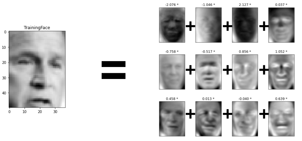
EigenFaces

Let’s assume that the input images are of size $n*n$. We represent these images in a higher dimensional vector space of dimension $n^2$. Note that this space of dimension $n^2$ might not be the perfect space to represent these vectors, for relatively few high-dimensional vectors consist of valid face images. If we’re able to effectively model a subspace which captures the key appearance characteristics of all the faces. In order to model this subspace or “face-space” we compute the k-dimensional subspace such that the projection of the data points onto the subspace has the largest variance among all k-dimensional subspaces.

This dimensionality reduction is performed using Principal Component Analysis. Principal component analysis is performed on a large set of images depicting different human faces, and the resultant eigenvectors are the required eigenfaces. Informally, eigenfaces can be considered a set of “standardized face ingredients”, derived from statistical analysis of many pictures of faces.

The original paper formalizing the method of eigenfaces can be found here

Go thorough the following links for better understanding:

🐼 Emotions

The Eigenface approach can be expanded to emotion identification as well. Go through the following papers for understanding how it is implemented:

🐼 Linear Discriminant Analysis and Fisherfaces

The issue with PCA projections is that they don’t track the labels of classes, hence not making them very optimal for classification. Another algorithm for dimensionality reduction called Linear Discriminant Analysis (LDA) finds a projection that keeps different classes far away from each other, hence also being helpful in classification problems. LDA allows for class discrimination by finding a projection that maximizes scatter between classes and minimizes scatter within classes.

Now, we can create a variation of Eigenfaces, called Fisherfaces which utilize Linear Discriminant Analysis for dimensionality reduction as opposed to PCA. Go through the following links to learn LDA and Fisherface methods:

Last section of Lecture 13 of CS131 for Mathematics Formulation of LDA
LDA introduction and python implementation
Face Recognition using Fisher Linear Discriminant Analysis (LDA)
Paper on LDA for Face Recognition

👾Day 2: Face Detection Models

Face Detection technologies have come a long way, with the Haar Cascades being the very first major breakthrough in the field followed by Dlib’s implementation of HoG(histogram of gradients).These methods used classical techniques, and with the rapid advancements in Deep learning, newer Face detectors came to rise, leaving behind the previous techniques in the ability to perform well in varied conditions such as lighting, occlusion, detecting faces having different expressions and scale, and their overall accuracy. Let us discuss two of these face detectors.

1.MTCNN

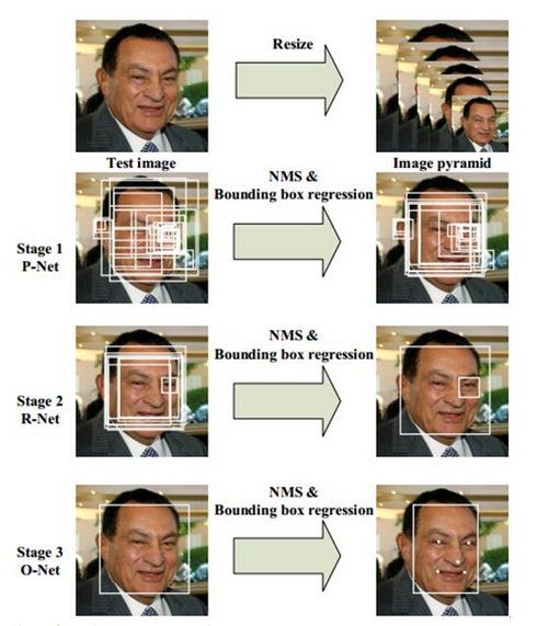
MTCNN Procedure

MTCNN or Multi-Task Cascaded Convolutional Neural Networks is a neural network which detects faces and facial landmarks on images. It was published in 2016 by Zhang et al(paper).

MTCNN uses a 3-stage neural network to detect not only the the face but also the facial landmarks (i.e. position of nose, eyes and the mouth). Firstly it creates multiple resized images to detect faces of different sizes. Then these images are passed on to the first stage of the model, the P-net or proposal net which as the name suggests proposes areas of interest to the next stage, the R-net or Refine network which filters the proposed detections. In the final stage, the O-net (output) takes the refined bounding boxes and does the final refinement to produce accurate results.

A short implementation of MTCNN is as follows-

before trying it you you will have to install mtcnn first by the following command

pip install mtcnn

# import the necessary libraries
import matplotlib.pyplot as plt
from mtcnn.mtcnn import MTCNN
from matplotlib.patches import Rectangle
from matplotlib.patches import Circle

# draw an image with detected objects
def draw_facebox(filename, result_list):
  data = plt.imread(filename)
  # plot the image
  plt.imshow(data)
  # get the context for drawing boxes
  ax = plt.gca()
  # plot each box
  for result in result_list:
    # get coordinates
    x, y, width, height = result['box']
    rect = plt.Rectangle((x, y), width, height,fill=False, color='orange')
    # draw the box
    ax.add_patch(rect)
    # draw the dots
    for key, value in result['keypoints'].items():
      dot = plt.Circle(value, radius=2, color='red') #change radius in accordance to 
      ax.add_patch(dot)
filename = r'test.jpg' #change to point to the image 
image = plt.imread(filename)
# detector is defined
detector = MTCNN()
# detect faces in the image
faces = detector.detect_faces(image)
# display faces on the original image
draw_facebox(filename, faces)
plt.show()

2.RetinaFace

RetinaFace

RetinaFace is state-of-the-art(SOTA) model developed to detect faces in adverse conditions and to outperform its predecessors . It has a reputation for being the most accurate of open-source face detection models.(paper). RetinaFace boasts one of the strongest face detection capabilities accounting for occlusion, small faces,and expressive faces.If you want a very robust face detector then RetinaFace is the go to choice

A short implementation of the following is given below and also remember to install the python-library by the following pip command

pip install git+https://github.com/hukkelas/DSFD-Pytorch-Inference.git

import cv2
import face_detection
# Initialize detector
detector = face_detection.build_detector("DSFDDetector", confidence_threshold=.5, nms_iou_threshold=.3)
# Read image
img = cv2.imread('test.jpg')
# Getting detections
faces = detector.detect(img)
# print(detections)
for result in faces:
    x, y, x1, y1 ,_ = result
    
    cv2.rectangle(img, (int(x), int(y)), (int(x1), int(y1)), (0, 0, 255), 2)
cv2.imshow("Image with Detected Faces", img)
cv2.waitKey(0)  # Wait for a key press to close the window
cv2.destroyAllWindows()

The two face detectors mentioned here are definitely not the only ones present. Here are some more that you are free to explore

YuNet
MediaPipe
Dual shot face detector
DNN module of openCV

👾Day 3: Face Recognition Models

If face detection answered the question “Is there a face in the image” then face recognition goes a step further and answers the question “Whose face is this?”. If you know about classification models, then you must be thinking that this task can be solved by using those, and while this is correct, classification models require a lot of data i.e. a lot of pictures of the same person to get trained on and get good results, which is seldom possible. If there is enough data to train your model, you could very well go along with a classification model.

One-Shot Learning

To tackle the problem of unavailability of data a technique called one shot learning is used.One shot learning aims to train models to recognize new categories of objects with only a single training example per category.This ability to learn about the data from just a single example is where its usefulness lies.One-Shot Learning is particularly valuable in scenarios where acquiring large datasets for every object category is impractical or expensive.This could include tasks like signature verification, identity confirmation, detecting new species,searching for similar products on the web and what not.

🔎 Read this article to get indepth understanding about one shot learning.

Siamese Networks

In the context of computer vision, Siamese neural networks are networks designed to compare similarities between two images and give a similarity score between 0 and 1.Siamese Neural Networks are a type of twin neural network that consists of two identical CNNs that share weights. It takes two input images, each is then processed by one of the networks to generate a feature vector, and then computes the distance between these vectors using a loss function. If the distance is small (less than a specified threshold), the images are classified as belonging to the same category.

🔎 Read this article to get a deeper understanding about Siamese Networks and try out their simple implementation by yourself.

👾Day 4: Visual Bag of Words

In face recognition, we learnt the pipeline of recognition, wherein we need to first represent them in the form of feature vectors which are mathematical representations of an image’s important features. We then create a space representation of the image to view the image values in a lower dimensional space. Every image is then converted into a set of coefficients and projected into the PCA space.

There can be various methods via we can reach this representation of the image in a lower dimensional space from the raw image. Today, we shall be exploring the Visual Bag of Words Approach.

Refer the Notes of Lecture 14 of CS131 and it’s lecture slides for the same. Moreover, the Bag of Visual Words concept is largely derived from the Bag of Words concept of NLP, so you can read this and this article to get a high level idea of the same before moving on to its visual counterpart.

Visual Bag of Words

🐼 Overview of Visual Bag of Words

🐯 Building Visual Vocabulary

Extract Relevant Features: Use various methods described earlier in the roadmap, like corner detection of SIFT features, splitting image into grid and using sub-images as features etc.
Clustering Features for Quantization: narrow down this large feature set into a smaller, less redundant set of common features. We can use clustering (KNN, Mean Shift or HAC) to identify similar features and use the cluster centers as the representation of the clusters.

The features thus extracted form out visual library.

🐯 Representing New Images by Visual Word Frequencies

We can represent every image in our dataset as a histogram of visual word or code-vector frequencies.
Then, we extract features from the new image (on which we’re training the model) and use our codebook to map the new image’s features to the indexes of the closest words (using some kind of similarity metric).
Each visual word (feature) can be assigned a weight on the basis of its commonality in various images, it’s frequency in a single type of image etc. We can give useless features low weights and the more important features higher weights.
Depending on the problem, train the model on the histograms thus created.

Go through the following resources for better understanding and implementation

🐼 Spatial Pyramid Matching

We’ve already explored Pyramids in the “Image Processing” weeks and worked enough on them. Now we shall apply the concept of Pyramids in exploiting spatial information of the image in the method of Bag of Words. You can go through the following resources to understand how it is done:

🐼 Naive Bayes

After producing a visual word histogram, Naive Bayes can be used to classify the histogram. You can try out other approaches as well, but Naive Bayes is widely used with BOVW in classification tasks.

👾Day 5 and 6: Motion and Tracking

Computer Vision is not all about static images, but also about videos - which are essentially multiple static images playing in a specific sequence at a particular frame rate (images or frames per second). In videos, we might be interested in location of objects, the time evolution of these locations (ie, the movement and motion of these objects), and this motion of objects with respect to other objects or markers (for instance whether a vehicle stops before a red light or crosses the zebra crossing while the light is red). For such applications, we require methods that can track the motion of pixels and features across various images, match particular features across multiple images to track the movement etc. Today, we’ll explore the pixel-level algorithms and methods for image tracking, and on tomorrow, we shall explore the abstractions (python libraries, modern methods etc) behind these methods.

For these two days, we shall be following Lecture notes of CS131 and the playlist on Optical Flow by Shree K. Nayar, a prof at Columbia University. This is a brilliant playlist of short videos which explains the concepts and mathematics in a pretty intuitive manner. Don’t be overwhelmed by the number of videos; the playlist contains videos as short as 4 minutes and the length of an average video is around 8-15 mins.

🐼 Motion

Go through Notes of Lecture 17 of CS131 for this subsection

The methods described below are pretty mathematically intensive and formulated in the form of a mathematics theorem (Assumption -> Modelling the problem-> Solving the Model). We’ll provide a logical explanation behind the algorithm in this roadmap without going into the math but you’re encouraged to go through the assumptions and equations as well.

Plus, don’t be intimidated by the equations and systems; because the mathematics involved in this section is pretty basic (High School Calculus and Linear Algebra at best), but just uses some intimidating notations. The core concepts are pretty simple

🐯 Optical Flow

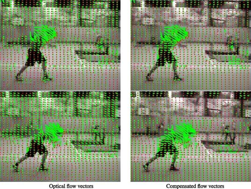
Optical Flow

Optical flow is the motion of objects between consecutive frames of sequence, caused by the relative movement between the object and camera. The flow can be modelled as the time and distance derivatives of the intensities of the pixels. The basic idea is to find the displacement vector $(u, v)$ for each pixel, which represents how much and in which direction the pixel has moved between the frames.

Watch the first three videos of this playlist for an understanding of mathematical modelling of optical flows
Read the first four sections of this Article to understand how optical flow is implemented

🐯 Lucas-Kanade method of Optical Flow

The basic assumption of this method is that for each pixel, the motion field and optical flow is constant within a small neighborhood around that pixel. Let’s call this neighborhood a ‘patch’. This means that we assume that all the pixels in this patch move in the same manner. - It assumes that the appearance (brightness) of these small patches doesn’t change much between frames. For example, if a part of an image is white, it will still be white in the next frame even if it has moved slightly.

The core idea is to track the movement of small blocks of pixels (patches) from one frame to the next. Imagine cutting out a small square from an image and then trying to find where that square moves in the next frame. This method works best when the movement between frames is small. The method assumes that the change in position of each pixel is relatively minor from one frame to the next. This assumption allows us to use the Taylor series expansion which shall not work for large changes in displacements. So, this method shall not work if the movements in a video are sudden and fast.

Go through the Fourth video of the playlist to understand the woeking of this method
You can not try to implement the rest of the sections of the Article referred in the last subsection.

Post this, you can go through the Horn-Schunk Method for Optical Flow from the lecture notes provided above.

🐯Pyramids and Coarse-to-Fine Flow Estimation

To expand the scope optical flows to fast videos as well, we introduce the concept of Coarse-to-Fine Flow Estimation using Image Pyramids. The baseline idea is that if we down-sample to image to a small enough resolution, then at some point, the movement of pixels between consecutive frames will become small enough to apply the Lucas Kande Method.

To understand how this works, go through the 5th and 6th videos of the playlist

🐼 Tracking

Go through Notes of Lecture 18 of CS131 for this subsection

🐯Structure from Motion

Tracking images might not only involve 2 dimensional tracking wherein an object is translating in 2 dimensions, but can also involve 3 dimensional movements like rotations, revolutions, and other random movements. We can track not only these movements, but also the movement of the camera, 3D structure of the environment we are capturing etc by extracting features and then mapping them.

For doing this, we must understand the structure of motion first and how these features and their tracking can be stored in form of numbers which the model can process.

Go through the 7th to 10th videos of the playlist for understanding the structure of motion problem and Feature Observation Matrix.

🐯Tomasi-Kanade Factorization

This method helps us in the factorization of the Observation Matrix, which in turn helps us to track the feature points. Watch the 11th video of the playlist to understand how it works and some real life applications of this factorization

🐯Object Tracking

Till now, we only tracked the points (pixels) of various objects in order to get some kind of information about their motion. In this section, we shall understand how we can track the whole object in any video. Note that our algorithm should be such that it is invariant to any kind of transformation (scaling, translation, rotation, skewing etc), as well as light intensity, for the same object in a video can be captured from various orientations and in various lightings.

Go through the 12th to 16th Videos of the playlist for understanding Object Tracking.

👾Day 7: Pose Estimations

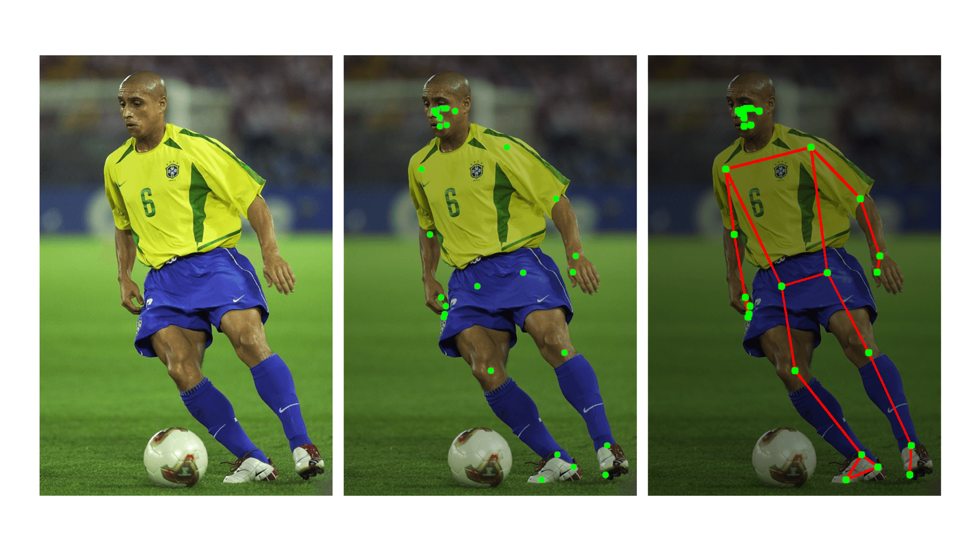
Post Estimation

Human pose estimation refers to the identification and classification of the poses of human body parts and joints in images or videos. In general, a model-based technique is used to represent and infer human body poses in 2D and 3D space. Essentially using this technique we find the coordinates of the human body joints like wrist, shoulder, knees, eyes, ears, ankles, and arms, which can describe a pose of a person. This finds its uses in Healthcare, AR and VR technologies, Animation, Character modeling and activity recognition.

To get started with pose estimation, I would suggest using MediaPipe or OpenPose for your first project. Here are some implementations to follow through for the same.

🦝Week 7: Intersections with NLP and Visual Attention

Week 6 largely concludes the conventional and fundamental Computer Vision applications and models ie recognition, detection and segmentation using CNNs and other ML algorithms. If you wish to stop here and specialize in a particular application like tracking, 3D Reconstruction, semantic segmentation etc, you can go ahead and explore research papers and cutting edge models; you have the fundamental knowledge of mathematics and computer vision to do so.

Week 7 onwards, we shall be focusing on upcoming trends for instance intersection of NLP and CV, Visual Attention, Gen AI, Graph NNs etc. This week, we shall start off with Visual Attention and CV X NLP. For this, you require some NLP background. If you’ve already completed the NLP roadmap, or have explored RNNs, LSTMs and Attention, you can skip a few days and directly skip to image captioning and Visual Attention and spend more time on these topics. Else, I’ve provided some background to these basic concepts and models in the following sections; which you can go through. Note that you won’t require an in-depth understanding and from scratch implementation of RNNs and LSTMs to understand the relevant concepts so even a high level understanding and basic mathematical knowledge works for this week.

Primary Resources for this week:

👾Day 1: Recurrent Neural Networks

A recurrent neural network (RNN) is a type of artificial neural network which uses sequential data or time series data. These deep learning algorithms are commonly used for ordinal or temporal problems, such as language translation, natural language processing (NLP), speech recognition, and image captioning; they are incorporated into popular applications such as Siri 👾👾👾, voice search, and Google Translate.

For an introduction to sequence learning problems, their need in Computer Vision, Computational Graphs and Recurrent Neural Networks: RNN Introduction by Prof Vineeth N Balasubramanian
Backpropagation Through Time in RNNs

This RNN cheatsheet by Stanford shall come in handy for revision

👾Day 2: LSTMs and GRUs

RNNs show multiple issues like Vanishing and Exploding gradient descent. To understand these issues better, follow the link: https://www.analyticsvidhya.com/blog/2021/07/lets-understand-the-problems-with-recurrent-neural-networks/

These issues are largely solved by Long Short Term Memory Models, which efficiently maintain short term as well as long term context, along with having an added functionality to eliminate information or memory if it’s no longer required.

But, LSTMs become exceedingly complex, requiring high compute, low interpretability and complex lines of code. Gates Recurrent Unit (GRUs) solve this issue by introducing Gates.

For understanding LSTMs and GRUs better, go through the following resources:

👾Day 3: Videos with CNNs and RNNs

Videos are sequential data structures, which are composed of a huge number of images which are interrelated to each other in a particular sequential order. So, to perform various tasks related to videos, it is convenient to use a combination of RNNs and CNNs which capture both, the advantage of convolution operation of images and the advantage of sequential data processing. Following resources delve deep into the topic:

Video Understanding using CNNs and RNNs by Prof Vineeth N Balasubramanian
[CS231n (2018) Lecture Slides](https://cs231n.stanford.edu/slides/2018/cs231n_2018_ds08.pdf
Video Classification using CNN-RNN architecture via Keras
Papers With Code Video Area enlists various subtasks within video tasks, like Video Understanding, Video Object Segmentation, Action Classification, Video Classification etc and has a repository of benchmark papers and their implementations. You can go through the subtasks and papers you find interesting.

👾Day 4: Visual Attention

The main purpose of attention mechanisms is to improve the model’s ability to focus on relevant parts of the input data (pay attention to them) when making predictions or generating outputs. This, in terms of Vision pans out as paying attention on specific parts of the images and specific features.

This video by StatQuest explains the need of Attention Models in Machine Learning
Visual intro to transformers and Attention In Transformers by 3B1B provide a visual understanding about Attention and Transformers (with respect to NLP)
Attention in Vision Models by Prof Vineeth N Balasubramanian provides a deeper understanding of how Attention is applied in Vision Models.

👾Day 5: Vision Transformers

Self-attention is a mechanism used to capture dependencies and relationships within input sequences. It allows the model to identify and weigh the importance of different parts of the input sequence by attending to itself. Self Attention is largely used in Vision Transformer architectures. The Transformer network is a architecture that relies entirely on self-attention mechanisms to compute representations of its input and output without using sequence-aligned RNNs or convolution.

This is a great article introducing essential topics in self attention like, positional encoding, query, value ,key ,etc without going deep into the math.\
Other Attention Models by Prof Vineeth N Balasubramanian shall introduce you to Neural Turing Machine, Deep Recurrent Attentive Writers and Spatial Transformers, which implement attention in different ways in their architectures.
Self Attention and Transformers by Prof Vineeth N Balasubramanian introduces you to multi-head attention and Vision Transformers.

👾Day 6: Image Captioning

An important application of Attention Mechanisms is Image Captioning. It is an intersection of NLP and CV in the sense that it has to extract various features from the image, label those features and generate a sequence of words which grammatically makes sense and is a relevant caption for the video provided. Note that for captioning an image, the model has to individually pay attention to certain components and extract information from them, for instance in an image where a “bird is flying in the sky”, it has to pay attention individually to: the bird, the wings of the bird to conclude that it is flying and the sky. Hence, attention models are highly useful in image captioning. You can go through the following videos to understand how the model works:

👾Day 7: Visual QnA and Visual Dialog

You’d have come across AI models which answer questions based on a particular image, or answer questions related to each other in succession. The prior is called Visual Question and Answer, whereas the latter is just an extension of Visual QnA and is called Visual Dialog. You’d have guessed that the models used to build such chatbots could require some attention to focus on specific parts of the image, some sort of Visual Feature Extraction for understanding the images, as well as some sequential architecture for generating the Natural Language. To understand how these things combine to perform such a task with decent accuracy, you can watch the video on Visual QA, Visual Dialog by Prof Vineeth N Balasubramanian

TYouhis shall conclude week 7. Note that you will not be able to implement the attention and transformer architectures because of the immense amount of time and mathematical knowledge required to implement them in code as well as the lack of compute to actually run these models. All you can do as of now is understand the logic and surface level math behind these models and if you’re interested in actually pursuing research in this domain, work on these model with some University or Company with strong enough compute :)

🦝Week 8: Generative Models: Prelude

Someway in your Artificial Intelligence journey you’d have come across models which “generate” information, for instance images, videos or texts after giving some kind of information to them in form of text prompts or images. For instance using GenAI, you can generate an image of the cute raccoon 🦝 near the academic area of IIT Kanpur going through trash 🗑️, or the image of a Tiger 🐯 standing on the stairs of the Open Air Theater. The input here, is the text, and the output is an image which maps to the text. These models, which are largely used for information generation are called Generative Models. In the next three weeks, and the last week, we shall be building upon Deep Generative Models, i.e. Generative Models which are built using Deep Learning architectures.

AI Generated image of the cute raccoon near the academic area of IIT Kanpur going through trash

The main resource that we shall follow for these four weeks is CS236: Deep Generative Models. Following are some important links: - Lecture Videos - Course Website - Official Lecture Notes - Syllabus and Lecture Slides - Lecture Slides GitHub

The course website of Cornell CS6785 also provides instructive resources.

This week shall require knowledge of PyTorch, sequential models like RNNs and Attention. We’ve already covered these topics, but if you require a refresher, you can go through:

👾Day 1: Introduction to Deep Generative Models

Constructing a Deep Generative Model essentially means finding a probability distribution in a space, and sampling from that probability distribution in order to give an output. Understand, that the dimensionality of the data in case of Generative Models will be extremely high, along with a high number of random variables. So some of the crucial questions we need to answer in order to build these generative models are:

How do we model the joint distribution of many random variables?
What is the right way to compare the probability distributions?

For an intro to DeepGen Models, go through the following resources:

CS236 Lecture 1 and its Lecture Slides
Intro to DeepGen Models

👾Day 2: Probability for Generative Models

DeepGen models shall be intensive in Probability Theory, Distributions and Linear Algebra, so for a refresher, go through the following documents:

To understand the representations of these probability distributions in terms of generative and discriminative models, go through:

Generative Models can now be divided into the following types:

Likelihood-Based Models:
1. Autoregressive Models
2. Latent Variable Models
3. Flow Models
4. Energy-Based Generative Models
5. Score-Based Generative Models
Likelihood-Free Models: Generative Adversarial Networks

We shall be learning about these models in detail in the next few weeks.

👾Day 3: Autoregressive Models

We begin our study into generative modeling with autoregressive models. Autoregressive models are a class of machine learning (ML) models that automatically predict the next component in a sequence by taking measurements from previous inputs in the sequence. In terms of Natural Language processing, this can look like generating the next word (or a probability distribution which provides the probability of the next word) given a sequence of words. In Image Generation, this can look like creating a probability distribution for predicting the color of the unknown pixel in a given image

For starters, go through this article to get a primitive understanding of Autoregressive Models in gen AI. Then, you can go through the following resources for an in depth understanding:

Some relevant research papers if you’re interested in a deep dive (These are not related to image generation, but important Autoregressive Models):

👾Day 4: Maximum Likelihood Learning, PixelCNN, PixelRNN

🐼 PixelCNN

PixelCNN is a CNN architecture that utilizes AutoRegressive Models for Image Generation. Go through the following articles to understand its architecture and implementation:

https://towardsdatascience.com/auto-regressive-generative-models-pixelrnn-pixelcnn-32d192911173
https://medium.com/game-of-bits/image-synthesis-using-pixel-cnn-based-autoregressive-generative-model-05179bf662ff

BONUS: If you’re interested in learning more about AutoRegressive Models, read this paper on Visual Autoregressive Modeling.

🐼 PixelRNN

Pixel-RNN presents a novel architecture with recurrent layers and residual connections that predicts pixels across the vertical and horizontal axes. The architecture models the joint distribution of pixels as a product of conditional distributions of horizontal and diagonal pixels. The model achieves state-of-the-art in the generation of natural images. To understand PixelRNN better, go through:

🐼 Maximum Likelihood Learning

Recall that when we learnt about Generalized Linear Models in the Machine Learning Roadmap, we used the Maximum Likelihood principle in order the train the model. We’ll be using the same principle in order to develop the concept of Maximum Likelihood Learning for Generative Models. For a refresher on Maximum Likelihood Principle and Probabilistic Interpretation of ML, go through:

Now, go through the CS236 Lecture 4 Slides and Lecture

👾Day 5: Latent Variable Models

🐼 Pros and Cons of AutoRegressive Models

Autoregressive models help in capturing sequential relations very effectively, but face the backlash of error propagation. Let’s understand these in detail

🐯 Advantages

Sequential Dependency Capture: Autoregressive models are excellent at capturing dependencies between data points in a sequence, making them highly effective for tasks like language modeling.
Exact Likelihood Computation: They allow for exact likelihood computation, which simplifies training and evaluation.
Flexibility: They can model complex distributions by conditioning each part of the data on the previous parts, providing high flexibility in the data they can generate.

🐯 Disadvantages

Slow Generation: Because data points are generated one at a time in sequence, generation can be slow, especially for long sequences.
Limited Parallelization and no scalability: Training and generation are inherently sequential, making it hard to leverage parallel computation, which slows down the process. Due do this, they are not scalable.
Error Propagation: Mistakes made early in the sequence can propagate and affect all subsequent outputs, potentially degrading the quality of the generated data.

This calls for a need of models which can capture more complex distributions, are able to parallelize its processes for scalability and is more interpretable. Herein, we introduce Latent Variable Models. Let’s break this term down and explore what Latent Variables ar first.

🐼 Latent Variables

Latent variables are variables that are not directly observed but are inferred from the observable data. Think of them as hidden factors or features that influence the observable data. For example, in image generation, the latent variables might represent abstract concepts like the shape, color, and style of objects in the image. To understand Latent Variables, go through this article

🐼 Latent Variable Models

LVMs are models that use latent variables to explain the observed data. These models assume that there is some underlying latent structure that generates the observed data. By learning this structure, the model can generate new data that is similar to the observed data.

During training, the model learns to encode images into a latent space, where each point in this space represents a set of latent variables. To generate a new image, the model samples a point in the latent space (i.e., a set of latent variables) and decodes it back into an image. Now, the latent space can be smooth and continuous, allowing for interpolation between points. This means you can generate new images by smoothly transitioning between different sets of latent variables.

To understand LVMs and the mathematics, go through these resources:

👾Day 6 to 7: Variational Autoencoders

Today, we shall explore an example of LVM: Variational Autoencoder. But before that, let’s take a look into Vanilla Autoencoders.

🐼 Vanilla Autoencoders

Autoencoders are a specialized class of algorithms that can learn efficient representations of input data with no need for labels. It is a class of artificial neural networks designed for unsupervised learning. Learning to compress and effectively represent input data without specific labels is the essential principle of an automatic decoder. This is accomplished using a two-fold structure that consists of an encoder and a decoder. The encoder transforms the input data into a reduced-dimensional representation, which is often referred to as “latent space” or “encoding”. From that representation, a decoder rebuilds the initial input. For the network to gain meaningful patterns in data, a process of encoding and decoding facilitates the definition of essential features.

Go through the following to learn more about autoencoders:

🐼 Variational Autoencoders

A variational autoencoder (VAE) provides a probabilistic manner for describing an observation in latent space. Thus, rather than building an encoder that outputs a single value to describe each latent state attribute, we’ll formulate our encoder to describe a probability distribution for each latent attribute. For a high level understanding of VAEs:

To get a visual understanding of VAEs, watch the following videos:

To understand VAEs from mathematical perspective, go through the following:

🐼 Applications and Variations of VAEs

It is really important for us to understand what exactly are the uses of VAEs. For this we should go through some resources explaining its application and how it is implemented. -https://medium.com/@saba99/navigating-the-world-of-variational-autoencoders-from-architecture-to-applications-05da018e0f61 -This pdf will also help. -This article may also help.

Variations of Variational Autoencoders (VAEs) extend the basic VAE framework to address specific challenges and enhance functionality. Conditional VAEs (CVAEs) incorporate additional information by conditioning the output on extra variables, making them effective for tasks like controlled data generation. Beta-VAEs introduce a weighting term to the KL divergence, promoting disentangled representations and making it easier to interpret the latent space. Disentangled VAEs aim to separate distinct factors of variation in the data, enhancing the model’s ability to generate and manipulate complex features independently. These variations expand the versatility of VAEs, enabling more precise control over generated outputs and improving their applicability across diverse machine learning tasks.

Here are some resources but it is not necessary have to have full proficiency on all of them. -This covers a lot of variations of VAEs. -Here is an implementation of CVAEs.

Some interesting research papers can be found below (obviously you won’t be able to cover these in the allotted time, so you can just put them in your reading list or devote more time to VAEs if you find them interesting):

🦝Week 9: Generative Models II

👾Day 1 to 3: Hands on VAEs

🐼 Implementing VAEs

Well going deep will involve learning with code. Go through this or this. First one contains implementation of VAEs with pytorch other with tensorflow. Go through it thoroughly. For those who want to delve in more details and maths here are the links to the original research paper and a revised version of it.

🐼 Some Mini Projects

These are some mini projects you can explore. It won’t be feasible to complete all the projects so you can just pick the one you find interesting.

🐯 Implement a Conditional VAE (CVAE) for fashion item generation

Dataset: Fashion-MNIST Use PyTorch or TensorFlow Architecture: Deeper encoder and decoder (4-5 layers each) Latent space dimension: 16 or 32 Condition on item category

🐯 Some Advanced training techniques

Implement KL annealing Use a cyclical annealing schedule Add a perceptual loss using a pre-trained classifier

🐯 Evaluation and visualization:

Reconstruct and generate images for each category Interpolate between different styles in latent space Quantitative evaluation: Frechet Inception Distance (FID)

👾Day 4 and 5: Normalizing Flow Models

🐼 Disadvantages of LVMs and VAEs

Approximate Inference: The learned latent space may not fully capture the underlying data distribution, reducing the accuracy of the model due to approximation of the posterior distribution using a variational distribution.
Intractable Likelihoods: Computing the exact likelihood of the data $p(x)$ in VAEs involves integrating over the latent variables, which is often intractable. In order to prevent this, VAEs maximize the Evidence Lower Bound (ELBO) instead of the true likelihood. Since ELBO might not be a tight bound on the true log-likelihood, this approximation can affect the quality of generative models.
Mode Collapse: VAEs can suffer from mode collapse, where the latent space fails to capture all modes of the data distribution, resulting in poor generative performance and missing diversity in generated samples.

Autoregressive models provide tractable likelihoods but no direct mechanism for learning features, whereas variational autoencoders can learn feature representations but have intractable marginal likelihoods.

Normalizing Flow models combines the best of both worlds, allowing both feature learning and tractable marginal likelihood estimation. Normalizing Flow models:

Allow for exact inference, as the likelihood can be computed explicitly. This happens via using a series of bijective mappings
Flow models provide a tractable likelihood function, which can be optimized directly without relying on variational approximations.
The invertible transformations in flow models can be highly flexible and expressive, allowing them to capture complex dependencies in the data.

How are these benefits achieved? We shall explore in the following sections.

🐼 Normalizing Flow Models

For a high-level idea about Normalizing Flow Models, go through these resources:

Intro to Flow Models by TDS
Gen Modelling through Flow Models
What are Normalizing Flows Video builds on some mathematics and provides visualizations
A short video on Normalizing Flows

After going through the above material, you should be ready to dive deep into the mathematics and formalism of NFMs:

If you’re brave enough 🦝, you can explore the Implementation of Normalizing Flow Models from scratch

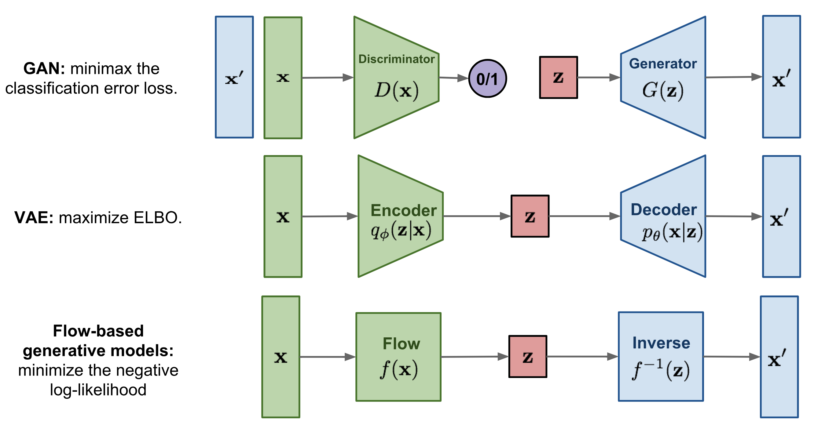
👾Day 6: Generative Adversarial Networks I

GANs v/s VAE v/s Flow Based Models

The next two days, we shall explore a new class of generative models: Generative Adversarial Networks. Unlike the previous models, GANs don’t utilize maximum likelihood for training but go for a likelihood-free training architecture. Let’s dive into GANs.

GANs are used for generative tasks and consist of 2 different models, a generator and a discriminator. The work of the discriminator is to distinguish the fake images from real images, and the task of the generator is to generate images so real that the discriminator is not able to distinguish.

🐼 Training of GANs:

This blog is based on the original GAN paper, but explains the topics in great details, it gets slightly mathematically involved at the end.

Today we will try to understand how actually the loss function of GANs work, this will help us understand how the generator knows it produces real-like images or not, how can we say that the discriminator is not able to distinguish, and how actually are there values updated.

🐼 GAN Maths

This shall be a good time to delve deep into the mathematics and theory of likelihood-free training algorithm and GANs in general

👾Day 7: Generative Adversarial Networks II

Today, we shall explore various types of GANs and some advanced methods. Before anything else, I’d like to emphasize on the absolutely insane number of GAN variants and the hilarious names allotted to them. You can find a list of majority of the named GANs in this repository called the “GAN Zoo”

🐼 DCGANs

DCGANs, or Deep Convolutional Generative Adversarial Networks, are a type of Generative Adversarial Network (GAN) that uses deep convolutional networks in both the generator and discriminator components.
The loss calculation and gradient descent in DCGANs are same as that in the vanilla GAN, only difference is in the architecture of the the Generator and Discriminator

Enough of theory , lets get our hands a little dirty!! This is a DCGAN tutorial by tensorflow, please do not get intimidated by the code,Use this Youtube video as a guide to understand the code better. Feel free to use google, AI assistance , or to contact us if you have problem understanding the code.

🐼 StackGAN

🐯 Architecture

The StackGAN architecture consists of two stages, each utilizing a separate GAN:

Stage-I GAN:
This first stage generates a low-resolution image based on the text description. It learns to produce a basic structure and rough colors that correspond to the input text.
Stage-II GAN:
Building upon the output of the Stage-I GAN, the Stage-II GAN takes the low-resolution image and refines it to generate a higher-resolution image that closely matches the details specified in the text description.

🐯 Why use Stacked Architecture?

By using a stacked architecture, StackGAN aims to overcome the limitations of directly generating high-resolution images from text, which can be challenging due to the complexity and detail involved. The approach of using two stages allows the network to progressively refine the generated images, leading to more detailed and realistic outputs. It has been found out in research, that generating high-resolution image directly from noise gives nonsensical outputs. Thus having a GAN that first generate low-resolution image, and then feeding this image rather than noise to our Stage-2, acts as a support and produces photo-realistic images.

Resources: Blog explaining architecture of StackGANs Video on Architecture

🦝 This would be a good time to go through CS236 Lecture 10 and Lecture Slides. This lectures dives deep into other types of GANs like f -GANs, Wasserstein GAN, BiGANs and CycleGANs

🦝 Some interesting research papers which you can go through in your free time:

🦝Week 10: Generative Models III

👾Day 1 and 2: Energy Based Models

In Autoregressive models, Variational Autoencoders and Normalizing Flow Models, model architectures are restricted which is a huge disadvantage for a generative model. For flexible model architectures, GANs were introduced, but in GANs, the likelihood is intractable, training is unstable, the models are hard to evaluate, and they have mode collapse issues. Today, we shall explore Energy based models which have:

Flexible model architectures
Stable training
Relatively high sample quality
Flexible composition

Energy-based models (EBMs) are another class of probabilistic models used in generative modelling to model the probability distribution of data. EBMs take inspiration from statistical mechanics and aim to model data distributions using an energy function. This function assigns low energy to likely observations and high energy to unlikely ones, mirroring physical systems where low-energy states are more probable. The fundamental concept involves expressing probabilities using a Boltzmann distribution, which normalizes the energy function.

Imagine a landscape of hills and valleys. In an EBM, each point in this landscape corresponds to a possible configuration of the variables (e.g., an image, a sequence of text). The height of the landscape at any point represents the energy of that configuration. The goal of training an EBM is to shape this landscape so that real data points are found in the valleys (low energy regions) and unrealistic data points are found on the hills (high energy regions). This is done by adjusting the parameters of the model to minimize the energy of real data points and increase the energy of other points. To get a high-level idea of Energy Based Models, go through the following links (in this order):

Now that you have a basic idea, let’s dive deep into the theory and math:

👾Day 3 and 4: Score Based Models

For a high-level idea about Score-Based models, go through:

Now, for diving deep into the theory and math:

Some interesting papers (optional), are as follows:

👾Day 5: Latent Representations and Evaluation

In any research field, evaluation is extremely important, as developments and improvisations on current models can only be done if they are evaluated. Hence, it is also important to know how to interpret and evaluate various Generative Models in order to find potential flaws (and if you’re lucky, breakthroughs 🦝). Go through CS236 Lecture 15 and its Lecture Slides

👾Day 6: Some Variants and Ensembles

In Machine Learning roadmap, we learnt about Ensembles, and how combining various models might lead to better accuracy as the shortcomings of one model can be compensated by the other if the ensembling is done in a correct manner. Today, we shall learn about various ensembles of the models we’ve studied throughout the last 3 weeks, namely PixelVAE, Autoregressive Flow, VAE+Flow Model Ensemble, Variational RNN, FlowGAN, Adversarial Autoencoder and $\beta$-VAE. We shall only be touching upon these topics, and you can delve deep into the specifics and mathematics if you’re interested in specific architectures. Go through CS236 Lecture Slides for learning about these models.

👾Day 7: Wrap Up and Further Readings

Revise, complete backlogs, take a break. If you’ve completed everything and are bored, you can go through the following:

🦝 Deep Gen Models and Boltzmann Machines 🦝 Advanced Tutorial on GANs 🦝 Generative Modeling by Estimating Gradients of the Data Distribution

🦝Week 11: Graph Neural Networks

Note that we shall not dive deep into the hardcore mathematics and theory of GNNs in this week, but just restrict ourselves to the basic math and practical aspects as GNNs are not really related to Computer Vision, but an important concept which involves convolution-like operations.

CN224W: Machine Learning with Graphs shall be our primary reference material for the week, but note that various advanced topics and methods which are not extremely useful from an implementation perspective will be skipped. If you wish to explore GNNs beyond the contents of this week, feel free to go through the all the contents of CN224W:

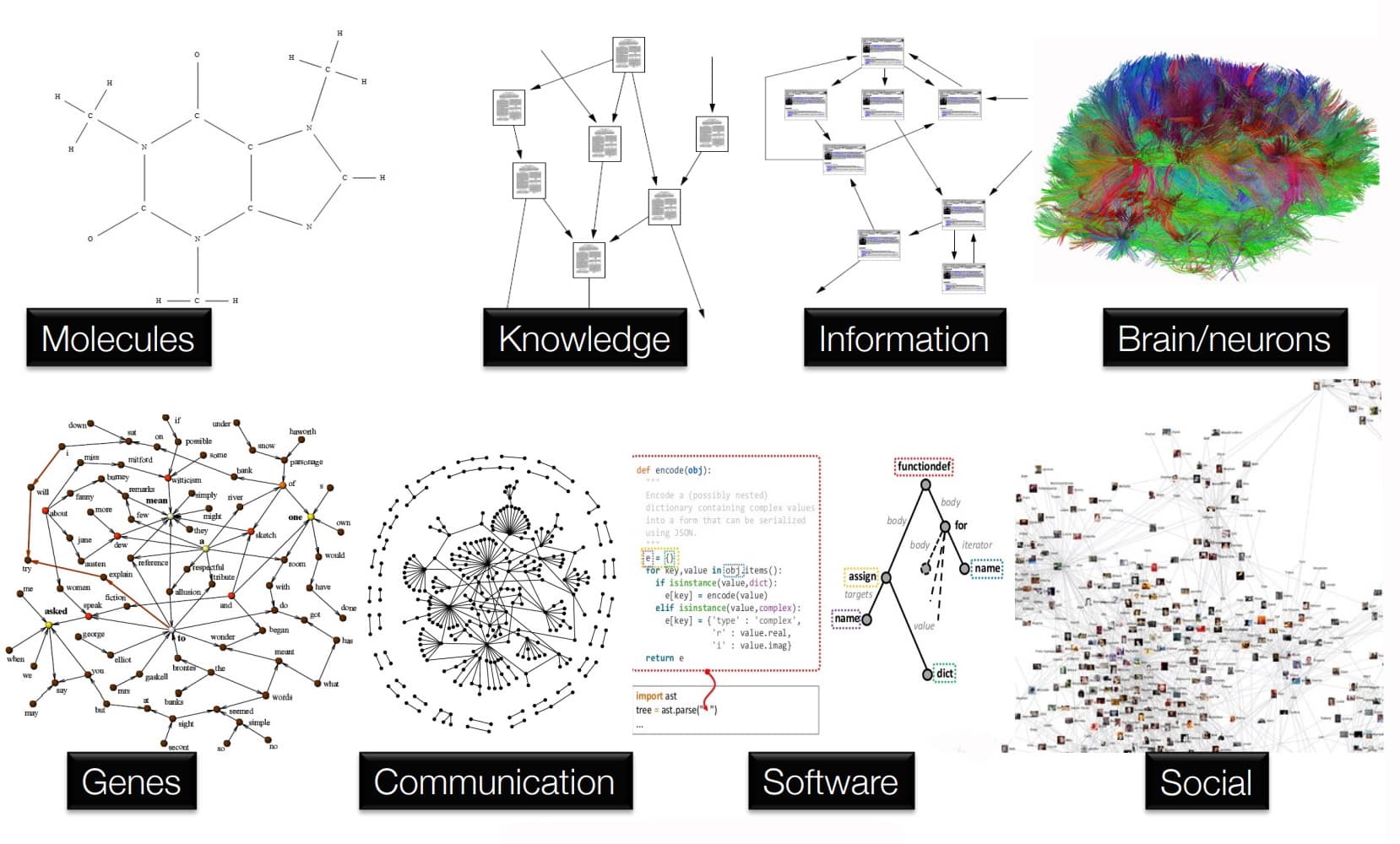
👾Day 1: Intuition, Introduction and Prelims

Graphs around us

🐼 Particles in a Box

Imagine a box filled with different types of molecules. Suppose you need train a model to predict:

Energy of a given molecule
Interaction Energy between two molecules
Total Energy of the system

Given an initial configuration and certain parameters like position of particles, types of particles, speed of particles etc.

Note that if we need to fit a model to predict the energy of a given molecule, it is a function of not only the features of that molecule, but also the molecules around it, their features and their proximity to the molecule under consideration. This means, in order to predict the target value for a given molecule, we must also consider the information from the other data points as well. Same applies for prediction of Interaction Energy between two molecules.

Let’s take a small detour from the problem at hand and analyze some models we have studied in the past.

More often than not, the input datapoints provided are related to each other in some way or the other. For instance, in time series data, a datapoint at a specific point of time might be related to the datapoints in history. For analyzing such data we use sequential data models called Recurrent Neural Networks. In images, one pixel is correlated to the pixels around it so we use Convolutions in order to capture the relationships between proximate pixels.

But if we consider this example, the positioning of the data points (ie, the molecule) is not as structured as an image which is extremely ordered in 3 Dimensions or like time series data which can me modelled in simply one dimension and plotted with respect to time. So, in order to model systems like the box with molecule in it, where the data points and correlations are not ordered, but connected in an unordered manner; we need a new data structure.

You must have heard about the data structure graph. Imagine a bunch of points, with some points connected to each other via “edges”. These points are called “Nodes” of the graph. Try to model the molecules in the box as a graph. What are the edges? Can we assign certain properties, or “weights” to these edges? Can we encode some information in these nodes? How do we then, apply the knowledge of neural networks to fit these graphs and predict the target variables? What kind of predictions can we do? Can we perform both, classification and regression?

These questions shall be answered slowly as you go through this week 🦝.

🐼 Graph as a Data Structure

To understand the Data Type Graph, it’s properties and types go through the following resources:

🐼 Graph-based Tasks

As you would have understood, complex data can be represented as a graph of relationships between objects. Such networks are a fundamental tool for modeling social, technological, and biological systems. In this section, we shall go through examples of graphs and various levels of problems.

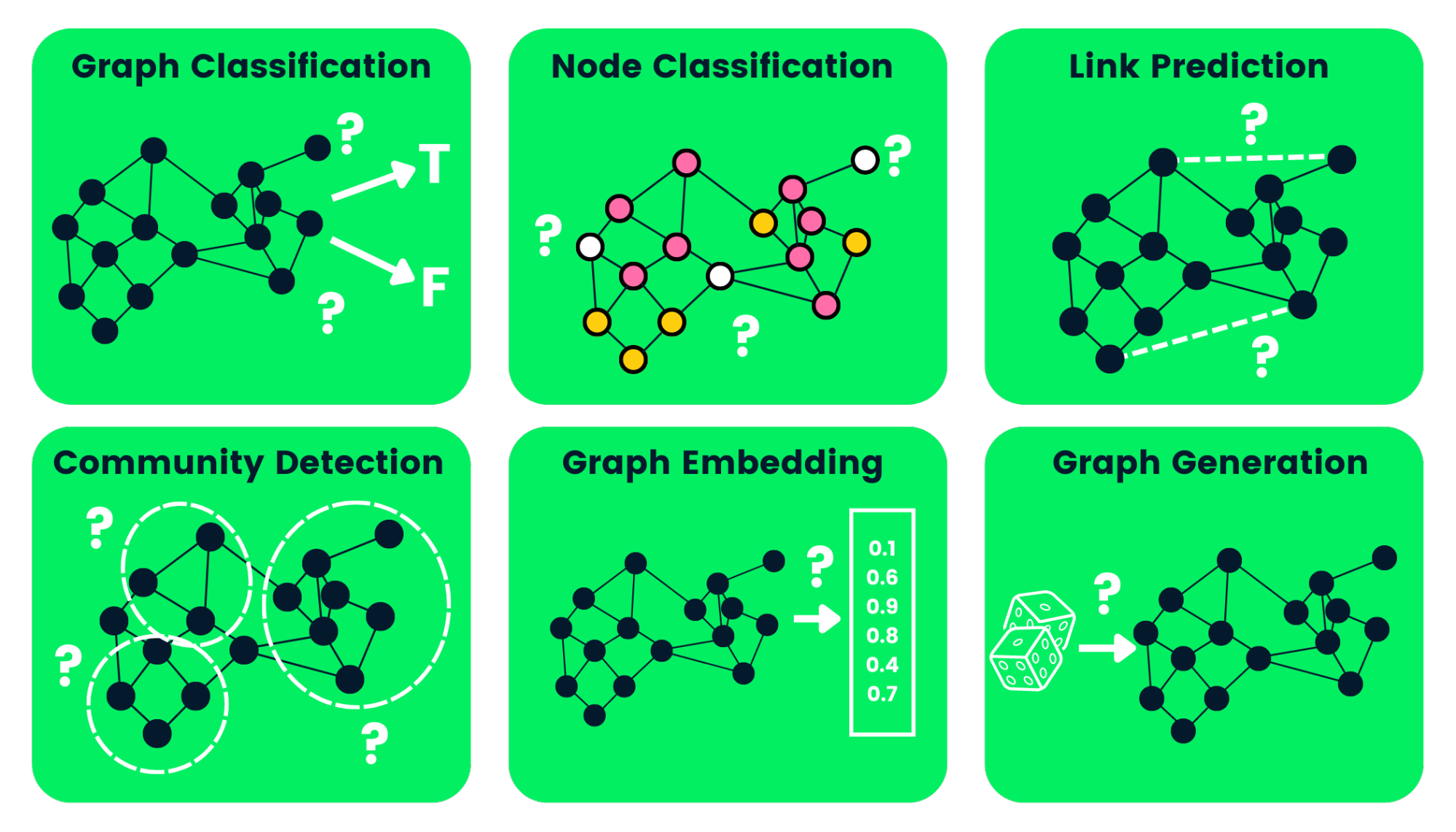
Tasks performed by GNNs

🐯 Graph-level task

In a graph-level task, our goal is to predict the property of an entire graph. For instance, finding the total energy of the box is a graph level task because the total energy is a function of all the molecules, and these molecules are modelled as a single graph with each molecule as a node and each significant enough inter-molecular interaction denoting an edge. This can be deemed as graph-level regression as our target variable is a continuous variable.

Another example: for a molecule represented as a graph, we might want to predict what the molecule smells like, or whether it will bind to a receptor implicated in a disease. This can be deemed as graph-level classification as our target variable is a continuous variable.

🐯 Node-level task

Node-level tasks are concerned with predicting the identity or role of each node within a graph. This could look like classifying a node, or evaluating the value of a specific property of a node, for instance finding the energy of individual molecule in the recurring example.

🐯 Edge-level task

Edge-level tasks can again be classified into edge regression and classification. An edge describes the relationship between 2 nodes, hence an edge classification might look like classifying the relationship between two nodes, and edge regression might look like determining the strength of relationship between the 2 nodes. For instance, in the molecules in a box example, calculating the interaction energy between the two molecules is an edge level regression.

🐯 Community-level task

Communities are subgraphs with certain properties. Within a large graph, there might exist smaller sub-graphs wherein the nodes are related in a particular manner. For instance in a graph which represents your class, there might be certain close friend groups. These close friend groups are communities. A community level task could be: identifying communities, classifying communities or assigning continuous values to communities.

Following is a great article to get started with graph as a data structure, their properties, need of Graph Neural Networks and their architecture: https://distill.pub/2021/gnn-intro/

Go through the following video for a visual understanding of Graph neural Networks: https://www.youtube.com/watch?v=GXhBEj1ZtE8&t=1s

Now, go through these Lecture Notesand the following video lectures:

👾Day 2: Node Embeddings and Message Passing

Yesterday we talked about how we can assign certain features to the node in order to capture their properties. The method via which this feature assignment happens is called Node Embeddings and usually involves assigning a feature vector to each node. Today we shall learn about Node Embeddings and a general architecture of GNNs. But first, lets learn more about graph features

🐼 More on Graph Features

🐯 Nodes

In order to characterize the properties and character of a node with respect to the given network (we shall use network and graph interchangeably), we require certain mathematical metrics.

Node Degree: Number the edges a node has. Describes how well-connected the node is in an absolute sense.
Node Centrality: A node might have varied levels of significance in a graph. Some nodes might be extremely important, while others might be dispensable. Node Degree does not consider this metric, but Node Centrality also tries to capture the importance of the nodes a given node is connected to.
Clustering Coefficient: By capturing the connectedness of the neighboring nodes of a given node, Clustering Coefficient tries to also consider the local structure of the graph while describing the node.
Graphlets

To understand these metrics better, go through this Video Lecture on Nodes and Node Properties

🐯 Edges

We defined various metrics to describe nodes in the last subsection. Similarly we can define metrics to describe edges, which in turn describe the strength of connection between 2 nodes. Go through this Video Lecture on Links/Edges and their Features to explore these metrics.

🐯 Graph

In CV, we studied about kernels which essentially are functions (matrices) applied on an array of pixels, and the Bag of Words concept. Kernels and BoW can also be generalized to graphs, and to understand how these extensions take place, you can watch this Video Lecture on Graph Kernels.

🐼 NetworkX

NetworkX is an important Python Library to deal with Networks (ie graphs) and presents numerous methods and algorithms to construct, evaluate, modify and cluster them. This Colab Notebook on NetworkX provides an instructive tutorial, and covers the concepts important for GNNs. If you want to explore this library more, you can go through its documentation.

🐼 Node Embeddings

Now that we’ve understood various metrics to describe nodes, edges and graphs, let’s understand how we can generate vector embeddings for nodes. Go through the following resources for the same:

Video Lecture on Node Embeddings
Video Lecture on Random Walk and node2vec algo
Video Lecture on Embedding Graphs
Lecture Slides on Node Embeddings
🐼 Message Passing and Node Classification

As you would have realized, the information of a given node influences the information of neighboring nodes based on the connectivity (edges) between them. This means, that we need some method to pass the information from one node to its neighboring nodes so that while evaluating a particular node we can consider the influence of other nodes as well. This is done by a method called Message Passing. For understanding how this happens and and how this is used in node-level classification, go through the following resources:
Video Lecture on Message Passing
Message Passing and Over-smoothing Blog
Colab Notebok on Node Embedding Pipeline

🐼 Relational, Iterative and Collective Classifiers

Go through the following resources to understand working of node-level classifiers:

🦝 Following are come insightful research papers you can go through:

👾Day 3: Graph Neural Networks

We’ll be referring to a lot of Deep Learning concepts which we explored in the Machine Learning Roadmap. Watch this Deep Learning Refresher for revision.

🐼 Intro to GNNs

An important part during message passing is learning the aggregation function, which takes in the message from the neighbors, and aggregates it to a singular value. This function is not necessarily linear and can have multiple non-linearities. Moreover, an important function is the transformation function which takes in the output from the aggregation function and combines that to the value of the target node. This transformation function is also to be learnt and can be non-linear. In order to learn these functions, Neural Networks are used. To understand how the aggregation and transformation functions are learnt and implemented in the graph, go through the following resources:

🐼 GNN Architectures

Now that we’ve understood the basic components required to build a GNN, let’s combine them in order understand the generalized architecture of GNNs. Go through the following Video Lectures for the same:

Go through this Colab notebook on implementing GraphSAGE layer for a hands on experience.

This Paper on SEMI-SUPERVISED CLASSIFICATION WITH GRAPH CONVOLUTIONAL NETWORKS will introduce you to a new type of GNNs: The Graph Convolution Networks which use the Convolution operation similar to that of CNNs.

👾Day 4: GNN Augmentations and Training GNNs

🐼 Graph Augmentations

Sometimes, the raw input graph might not be the best input for the GNN, since if the graph is too sparse, information passing might be inefficient. Else, if the graph is way too dense, information passing might be costly and redundant. Hence, it is advised to augment the graphs before passing them through GNNs. For understanding how these augmentations can be done in various cases, watch this Video lecture on Graph Augmentation

🐼 GNN Pipeline and Training

Let’s conclude the fundamentals of GNNs by understanding how to train a GNN, what are the evaluation metrics and how are they used and how a basic GNN pipeline looks like:

🐼 Implementing GNNs

Now that we’ve understood the workings of GNNs and its architecture, let’s try to implement some GNN architectures:

🦝 Following are some insightful research papers you can optionally go through:

If you’re interested in how Attention can be implemented in GNNs, go through the following paper and colab notebook:

👾Day 5: ML with Heterogeneous Graphs, Knowledge Graphs

Sometimes, the nodes in a graph don’t represent the same class of objects, but contain different classes and entities. Such graphs are called Heterogeneous graphs. A form of Heterogeneous graphs are knowledge graphs which are huge networks containing numerous entities (from different classes) and relationships. A knowledge graph is essentially a graph-structured knowledge base that stores factual information in the form of relationship between entities, enabling the modeling of real world entities and their relations, and consequently powering search engines, natural language understanding systems and more recently recommender systems.

Until now we’ve only explored the node embedding methods for Homogeneous graphs. Since now the nodes have different entity classes, it will not be effective to use the same kind of message passing as we used in homogeneous to model knowledge graphs. Hence, we shall also explore Knowledge Graph Embeddings today.

Go through the following resources (in this order):

Once you’re done with the theory, you can go through this Colab notebook on working with Heterogeneous Graphs and try to implement it on your own.

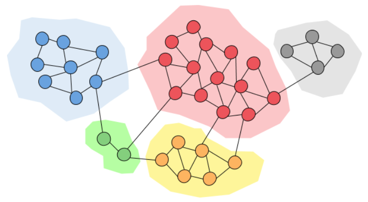
👾Day 6: Neural Subgraphs and Communities

Communities in a Graph

On Day 1 of this week, we mildly introduced you to Communities and Sub-Graphs and how GNN can also he helpful in various Community-based tasks. Today, we shall understand the modelling techniques and properties of of subgraphs, how to set up GNNs for community-based tasks, what kind of loss functions are used for subgraph matching and how communities can be detected using GNNs. Go through the following resources for the same:

👾Day 7: GNNs for Recommender Systems

Graphs are a primary representation tool in various Recommender Systems, and the advent of GNNs have improved the accuracy and efficiency of recommender systems multifold. For understanding how Graphs are utilized in these Recommender Systems and what kind of embeddings and loss functions are utilized, go through the following slides and resources:

This shall conclude your time with Graph Neural Networks. If you wish to explore more, as stated earlier feel free to explore all the resources of Stanford CS224W Course and go through cutting edge research papers.

🦝Week 12: Diffusion Models

In week 10, we talked about various types of Generative Models, and concluded with Score Based Models. This week, we shall build upon our knowledge of these generative models and try to understand the most famous DeepGen AI architecture: Diffusion Models.

👾Day 1: Introduction to Diffusion Models

So far we’ve studied about various Generative Models, for instance GANs, Autoencoders, Variational Autoencoders etc. Diffusion is another type of Generative Model that work by destroying training data through the successive addition of Gaussian noise, and then learning to recover the data by reversing this noising process. After training, we can use the Diffusion Model to generate data by simply passing randomly sampled noise through the learned denoising process.

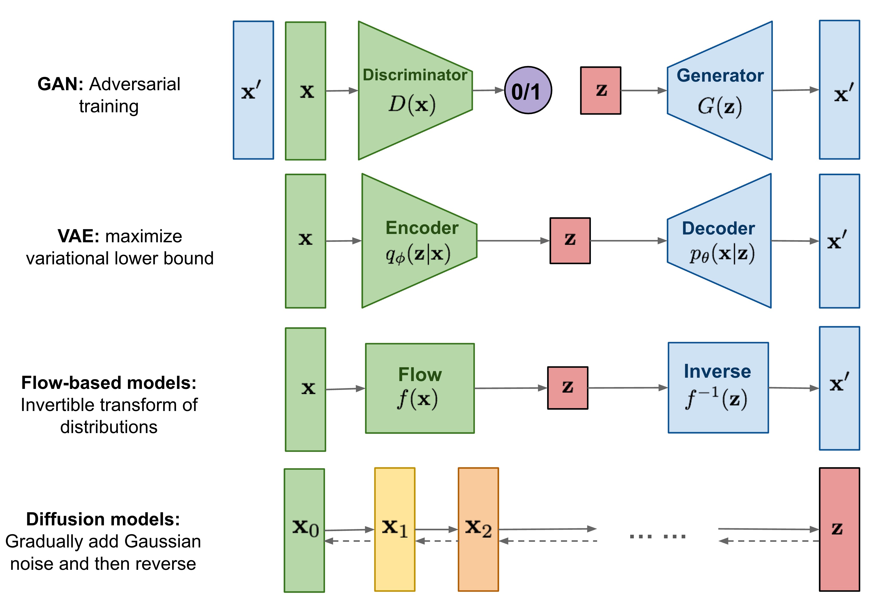
GANs v/s VAEs v/s Flow-Models v/s Diffusion Models

For understanding the difference between Diffusion and Auto Regression, watch the following video: https://www.youtube.com/watch?v=zc5NTeJbk-k&t=752s

For a high level understaning of functioning of Stable Diffusion (a famous diffusion model), follow this link: https://www.youtube.com/watch?v=1CIpzeNxIhU

Folloing is a brief introduction to Diffusion Models: https://www.assemblyai.com/blog/diffusion-models-for-machine-learning-introduction/

👾Day 2: Physics and Probability

The core concept behind diffusion models has been derived from Thermodynamics. Understanding the same would provide an intuitive understadning of how Diffusion Model work. The following link provides an explanation regarding the same: https://www.assemblyai.com/blog/how-physics-advanced-generative-ai/#generative-ai-with-thermodynamics

Understanding the mathematics behind Diffusion Models requires some additional prerequisites. I’m assuming that you’ve gone through the mathematical prerequisites for ML highlighted in the ML Roadmap. Go through the following articles and videos for the same:

👾Day 3: Score-Based Generative Models

Score-Based Generative Models are a class of generative models that use the score function to estimate the likelihood of data samples. The score function, also known as the gradient of the log-likelihood with respect to the data, provides essential information about the local structure of the data distribution. SGMs use the score function to estimate the data’s probability density at any given point. This allows them to effectively model complex and high-dimensional data distributions. Although the score function can be computed analytically for some probability distributions, it is often estimated using automatic differentiation and neural networks.

For better understanding, go through the blog post by Yang Song: https://yang-song.net/blog/2021/score/

Now, go through CS236 Lecture 16 and its Lecture Slides, along with CS236 Lecture 17

You can use this blog by Lilian Weng as a supplementary material to understand the mathematics.

(Tip: For delving deep into a topic, its usually a nice practice to go through the relevant references of the article you’re reading)

👾Day 4: Denoising Diffusion Probabilistic Models

DDPMs are a type of diffusion model used for probabilistic data generation. As mentioned earlier, diffusion models generate data by applying transformations to random noise. DDPMs, in particular, operate by simulating a diffusion process that transforms noisy data into clean data samples. During inference (generation), DDPMs start with noisy data (e.g., noisy images) and iteratively apply the learned transformations in reverse to obtain denoised and realistic data samples.

DDPMs are particularly effective for image-denoising tasks. They can effectively remove noise from corrupted images and produce visually appealing denoised versions. Moreover, DDPMs can also be used for image inpainting and super-resolution, among other applications

For a greater understanding of how DDPMs work, go through the following links:

👾Day 5: Discrete Models

Modelling Discrete data is important, for various variables in real world are not actually continuous, but discrete in nature. For understanding discrete variants of various models (DDPMs, Diffusion Models, LVMs), go through the following resources:

👾Day 6: Implementing Diffusion Model

Considering we’re largely done with the introductory material for Diffucion Models, let’s get our hands dirty with implementing DDPMs:

👾Day 7: Autoregressive Diffusion Model (ARDM)

AutoRegressive Diffusion Model capture the benefits of both, Autoregressive models and Diffusion Models. Unlike standard ARMs, they do not require causal masking of model representations, and can be trained using an efficient objective similar to modern probabilistic diffusion models that scales favourably to highly-dimensional data. At test time, ARDMs support parallel generation which can be adapted to fit any given generation budget. We find that ARDMs require significantly fewer steps than discrete diffusion models to attain the same performance. Finally, we apply ARDMs to lossless compression, and show that they are uniquely suited to this task. Contrary to existing approaches based on bits-back coding, ARDMs. Go through the following links for a better understanding:

🦝What Next?

You can explore the List of Courses offered by Stanford Vision Lab in order to explore various advanced topics in Computer Vision

👾3 Dimensional Reconstruction and Recognition

In this roadmap, we largely covered 2D problems. You can explore topics in 3D Reconstruction and Recognition as well. Following might be a good starting point:

CS231A: CV, From 3D Reconstruction to Recognition

👾Advanced Topics

CS331: Advanced Topics in CV covers a number of advanced topics and research papers in the field of CV

Syllabus and Lecture Notes

👾Applications in Robotics

Computer Vision is used intensively in Robotics due to the need for the bot to interact with the environment. This course might be a good starting point:

CS331B: Interactive Simulation for Robot Learning

Course Website

👾 Probabilistic Graph Models

Probabilistic graphical models are a powerful framework for representing complex domains using probability distributions, with numerous applications in machine learning, computer vision, natural language processing and computational biology. The CS228 Probabilistic Graphical Models course might be a good starting point to explore this domain:

Course Website
Notes
Probabilistic Graphical Models: Principles and Techniques by Daphne Koller and Nir Friedman

👾 Graph Neural Networks

In the roadmap, we only provided a brief intro to GNNs. Following are some resources to expand your knowledge:

BTW, some interesting personal websites and blog-sites: 🦝 https://yang-song.net/ 🦝 https://lilianweng.github.io/ 🦝 https://fanpu.io/ 🦝 https://sassafras13.github.io/

Contributors

Aarush Singh Kushwaha | +91 96432 16563
Anirudh Singh | +91 6397 561 276
Himanshu Sharma | +91 99996 33455
Kshitij Gupta | +91 98976 05316
Suyash Kumar | +91 98071 99316

Computer Vision Roadmap 🦝

Roadmap to Computer Vision 🦝

🦝 Meta-Knowledge

🦝 Meta-Roadmap

🦝 Recurring Resources

🦝 Table of Contents

🦝 Week 1: Image Processing I

🦝 Week 2: Image Processing II

🦝 Week 3: Convolutional Neural Networks

🦝 Week 4: Segmentation and CNN Architectures

🦝Week 5: Object Recognition and Detection

🦝Week 6: Some Important Applications

🦝Week 7: Intersections with NLP and Visual Attention

🦝Week 8: Generative Models: Prelude

🦝Week 9: Generative Models II

🦝Week 10: Generative Models III

🦝Week 11: Graph Neural Networks

🦝Week 12: Diffusion Models

🦝 Week 1: Image Processing I

👾Day 1: Digital Images and Linear Algebra Review

👾Day 2: Color and Color Spaces

👾Day 3: Pixels, Filters and Convolutions

🐼Image Histograms

🐼Image Filters

🐼 Convolutions

👾Day 4: OpenCV 101

👾Day 5: Thresholding

👾Day 6: Morphological Transformations and Edge Detection

🐼 Binary Image Processing

🐼 Edge Detection

👾Day 7: Fourier Transforms and Contours

🐼Fourier Transforms

🐼 Contours

🦝 Week 2: Image Processing II

👾Day 1: Key points, Image Features, Feature Descriptors

🐼 Keypoints

🐼 Image Registration

🐼 Robust feature matching through RANSAC

🐼 Scale Invariant Keypoint Detection

🐼 Scale Invariant Feature Transform (SIFT) Algorithm

🐼 Histogram of Oriented Gradients (HOG)

👾Day 2: Pyramids and Wavelets

🐼Pyramids

🐼Sub-Band Coding

🐼Wavelets and Multi-Resolution Processing

👾Day 3: Resizing Algorithms

👾Day 4: Strides and Padding

👾Day 5: Geometric Transformations and Geometry Detection

🐼 Geometric Transformations

🐯Warping

🐼 Contour Matching

🐯 Hu Moments

🐯Contour Detection and Matching

🐼 Line, Circle and Blob Detection

🐼 Finding the Raccoon 🦝🥺

👾Day 6 and 7: Practice and Hand-on Stuff

🐼 Face Detection and Recognition

🐼 Edge Detection and Image Filtering

🐼 Barcode and QR Code Scanner

🦝 Week 3: Convolutional Neural Networks

👾Day 1: Intro to CNNs for Visual Recognition

🐼What are CNNs?

🐼Key Components of CNNs

🐼Convolutional Layers

👾Day 2: Refresher: Loss Functions, Optimization and BackProp

👾Day 3: Pooling, FC Layers, Activation Functions

🐼 Pooling Layers

🐼 Fully Connected Layers

🐼 Activation Functions

🐼 Connecting the Dots: The CNN Architecture

👾Day 4: Data Preprocessing, Regularization, Batch Norm, HyperTuning

🐼 Data Preprocessing

🐼 Regularization

👾Day 5: Data Augmentation, Optimizers Review

🐼 Data Augmentation

🐼 Optimizers Review and Second-Order Optimization

👾Day 6: Deep Learning Hardware and Frameworks

🐼CPU v/s GPU

🐼Computational Graphs DL Frameworks

👾Day 7: Hands on Stuff