Kolmogorov–Arnold Networks

Neural Networks are largely seen as backboxes which magically provide the required output for a particular input, highlighting that they are not really interpretable and the whole process of training and tracking the learning of any neural network is unintuitive. That is, even if a Neural Network can provide correct answers, we cannot understand the reasons why it makes these decisions. When I say “neural networks”, I primarily refer to a class of networks called “Multi Layered Perceptron” (MLPs), which are modelled on the basis of the “Universal Approximation Theorem” (UAT), and use linear weight and bias matrices as trainable parameters. All the learning algorithms today are mostly based on MLPs and the UAT.

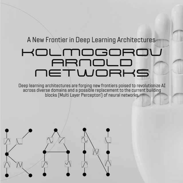
A few weeks ago, researchers from MIT, CalTech and Northeastern University released a paper which tries to use the Kolmogorov–Arnold Representation Theorem, trainable activation functions and B-Splines in order to model a network namely, the Kolmogorov–Arnold Network (KAN). This Network Architecture proposes a more interpretable and potentially effective alternative to MLPs. In this blog, we’ll be discussing about the architecture of KANs and what differentiates it from MLPs; along with the supplementary concepts required to build the mathematical framework and an intuition behind the Network.

Some of the aforementioned terms might sound way too intimidating at the first look, but they are just simple functions represented with such a complex level of Greek notation (That’s what mathematicians do 🙃) that they look more like alien scriptures than mathematics. But don’t worry, in this blog I’d try to break down these mathematically intensive theorems and architectures built on them in a much intuitive manner. Note, that the purpose of this blog is not only to provide intuition but to build that intuition into a mathematical rigor. Moreover, I’ve tried to keep this as sparse as possible, but cover all the important aspects, so this might be a mildly long read. The blog assumes basic knowledge about Highschool Calculus, Linear Models, Neural Networks and Activation Functions. A quick read, or binging the first four videos of the 3B1B playlist on Neural Networks over a Dark Chocolate will be enough.

Chapter 1| The Status Quo: Multi Layered Perceptron

If you’re already well versed with the Universal Approximation Theorem, MLP Architecture and potential roadblocks with the same, you can skip to Chapter 2

1.1| Universal Approximation Theorem

Ever wondered why and how MLPs held their ground as the default foundational building block of basically every Deep Neural Network ranging from simple classification models to those sophisticated LLMs for easily over 20 years? If you really think about it, with the rapid pace and remarkable progress in Machine Learning, its pretty crazy for MLPs to not see any contender for its position for such a long time.this just goes to show how good they actually are and how difficult it is to find something better.
Their strength lies in their foundation itself that is the Universal Approximation Theorem. Universal Approximation theorem states that no matter what a function $y=F(x)$ be ,there exists a series of neural nets $\phi _{1},\phi _{2},…$ such that eventually $\phi _{n}\rightarrow f(x)$.Okay lets end the mathematical jargon here and let me try to tell you what it aims to do. First imagine any non linear continuous function of $x$ (say a sine curve) , now try to draw line segments on that curve such that those line segments fit the curve as neatly as they can. In other words define a function that says if $x \in (a,b)$ then follow this straight line such that each $(a,b)$ do not intersect each other and cover all possible values of $x$.

1.2| MLP Architecture

We have been discussing MLPs for a very long time here, but do you know what they actually are? Multi Layer Perceptons are really just a type of artificial neural network consisting of multiple layers of neurons. The neurons in MLP typically use nonlinear activation functions, allowing the network to learn complex patterns in data. You might actually be very familiar with their architecture that is just a feed-forward neural network consisting of an input layer, hidden layers and finally an output layer all linked through nonlinear activation functions. Well, the only difference between ANN and MLP is that MLPs always have nonlinear activation functions while ANNs may or may not use them. If you are familiar with machine learning all this must already be known to you, but in case you aren’t here is a pretty great video for you to understand all the stuff related to ANNs along with the essential maths.

1.3| Issues with MLP

Even though MLPs may be the best solution to most of the problems we aim to solve in machine learning they do have their own disadvantages.

1. Vanishing/Exploding Gradients: MLPs use the backpropagation algorithm to train themselves. During this training gradients can become very small (vanishing) or very large (exploding) as they travel through multiple layers. This is a very remarkable drawback of using MLPs because as we add more and more hidden layers to deal with more complex data vanishing and exploding gradients make it very ineffective and inefficient for network to learn.
2. Hyperparameter Tuning: MLPs require careful tuning of hyperparameters like learning rate, number of layers and neurons, and activation functions. Believe me when I say that hyperparameter tuning is quite a process, turn the learning rate higher and here come the exploding gradients, turn it down and now the network doesn’t converge. Too few hidden layers and the network doesn’t learns anything and too much of them just for the model to over-fit the data.There are techniques and rules-of-thumb that help but they cannot dispose off the problem and even with their help there is essentially no way to determine if the hyperparameters you have used to train the best model you got is actually the best possible model (its pretty sad imo).
3. Interpretability: Understanding how MLPs arrive at their decisions can be difficult specially when there are multiple layers but understanding them is also very essential for several reasons such as getting insight into the data(crucial for research purposes), to improve the model , and to check the the fairness and biases of the network. The passing of data between weights and activation functions makes it a challenge to interpret the inner workings of the network. Its like the game where we had to connect dots to reveal a picture but the dots are all jumbled and there are a lot of them(really a lot) and then they also connect to multiple dots.

Chapter 2| The Prequels: KART and Splines

2.1| Kolmogorov–Arnold Representation Theorem

The Theorem can be summed up in the following simply equation:

\(f(X) = f(x_1, x_2, ..., x_n) = \sum_{q=0}^{2n} \Phi _q \left(\sum_{p=1}^{n} \phi _{q,p} (x_p) \right)\) where $\phi_{p,q}: [0,1] \rightarrow \mathbb{R}$ and $\Phi_{q}: \mathbb{R} \rightarrow \mathbb{R}$

This notation at a surface level might seem to be extremely complex (Honestly, I was flabbergasted when I first saw it), but it simply states that any multivariate continuous function (here, $f(X)$) can be represented as a superposition of continuous functions of one variable and the additive operation. Let’s break it down.

Let’s ignore the outer summation for a bit and focus on the inner summation. \(\sum_{p=1}^{n} \phi _p (x_p) = \phi _1 (x_1) + \phi _2 (x_2) + ... + \phi _n (x_n)\) here, $\phi _p (x_p)$ is just an arbitrary univariate function (called the inner function) in $x_p$ and we are summing $n$ such univariate functions in $n$ different variables.

$\Phi_{q}$ is also a univariate function, taking \(\sum_{p=1}^{n} \phi _{q,p}(x_p)\) as a whole as a single variable. Note that when we apply $\Phi_{q}$ on the inner function, we achieve a mixing a variables. That is, we can have terms line $x_{1}^{a}x_{2}^{b}$ or $(x_3)^{3}cos(x_2)sin(x_1)$ or $ e^{x_{2}^2 + x_{3}^{3}}sin(x_{1})$ as our in our output. This allows for a wide variety and forms of terms which might be very similar to the final function. Note, that we might not be able to achieve the $f(X)$ in a single iterations, so we superimpose 2n+1 such functions in order to obtain $f(X)$ .

The proof as to why we will necessarily be able to decompose $f(X)$ into such a superposition and why we need $2n+1$ functions in the outer summation is beyond the scope of this blog. Moreover, there exist variations of the KART, for instance replacement of the outer functions $\Phi_{q}$ with a single outer function $\Phi$ by George Lorentz, replacement of the inner functions $\phi_{q,p}$ by one single inner function with an appropriate shift in its argument by David Sprecher and generalization of KART by Phillip A. Ostrand via compact metric spaces. Again, these variations are not really important for understanding KANs, but present pretty interesting manipulations and applications (might cover the proofs, variations and results in another blog later 🥰)

The KART in a way tries to approximate the function $f(X)$ via decomposition. Since in machine learning models, the main task loosely is to find a function that can approximate the behavior of the system we are trying to model (called the “Hypothesis function”), this decomposition might somewhat be helpful in approximation of the function. Even before the extremely popular 2024 paper on KANs, multiple attempts have been made to implement the KART to develop network architectures, but they have largely failed in doing so. Why? We shall explore that in the next section.

2.2| “Kolmogorov’s Theorem is Irrelevant”, lmao

In 1989, Girosi and Poggio released a paper which literally, without hesitation claimed that “Kolmogorov’s Theorem is Irrelevant” ☠️. We’ll cover the underlying reasons behind this claim in this section.

Girosi and Poggio primarily claimed 2 fallacies: 1) Non Smoothness of Functions: It is claimed that the inner functions of KART are not necessarily smooth. Here, I shall not delve into the mathematical definition of smooth but at a high level, these are functions whose derivates can be calculated till a sufficient depth (simply put, the curves look smooth 👍). Hence, Kolmogorov’s theorem relies on constructing inner functions that are highly non-smooth. In the context of neural networks, smooth activation functions are preferred because they facilitate gradient-based optimization techniques such as backpropagation; because multiple partial derivatives are necessary for backpropagation. Non-smooth functions, on the other hand, introduce difficulties in optimization and can lead to poor performance in learning tasks. This is a major roadblock. 3) Lack of parameterization: The functions provided by Kolmogorov’s theorem are not parameterized in a form that can be easily adjusted or learned through data. MLPs can easily be parameterized via weights as biases; but it becomes increasingly difficult to parameterize a KART function in such a way that at each iteration, it can be altered on the basis of some learning. Neural networks require functions with parameters that can be tuned during training to approximate the desired outputs. The lack of such parameterization in KART functions makes them impractical for real-world neural network applications.

Had KART actually been irrelevant and it’s implementation in a network actually not been feasible, I’d not have been writing this blog. So obviously, the new paper presents methods to overcome these problems, including Non Linear and Learnable Activation Functions and the implementation of the same via B-Splines. Before delving into the actual model, let’s understand Splines.

2.3| Beautiful Curves: Splines 🥰

2.3.1| Splines as threads

Imagine a thread which can be easily deformed to change its shape. Stretch it out to form a line segment and now select 4 points (not the endpoints) A, B, C and D in that order on the curve. Observe the shape of the curve between the extreme points (A and D). Take any point (say, B) and alter the shape of the curve by moving the curve at that point, keeping other points fixed. The line now becomes a curve. Such a curve is called a spline. Observe that by altering the 4 points in various fashions, you can create infinitely many curves, and these curves will just be a function of the initial and final positions of the points. These fixed points (A, B, C and D) are called control points. These control points help to “pull” the curve (spline) to its desired shape and in this example, the shape is determied via the natural Tension in the wire.

Note that this is just an example of a spline which follows certain properties. We can define as to HOW the spline is constructed from its control points via and algorithm; and this gives rise to different types of splines. Moreover, it is not necessary that the control points always lie on the spline; they might or might not lie on it. When one or many points lie on the spline, we say that the spline “interpolates” the point. In the following sub sections, we’ll explore various properties, advantages and classes of splines and finally conclude with B-Splines.

2.3.2| Pice Wise Cubic Curves and C1 Continuity

Given 4 points in the cartesian plane, can you find an equation which passes through those 4 points? Just assume a cubic equation, substitute the values and solve the resulting system of 4 linear equations. What about 2 points and the slope of tangents of those points? Again, you can assume a cubic equation, differentiate it to get the slope of the tangent, substitute values in the cubic euqation and equation of slope and find the coefficients.

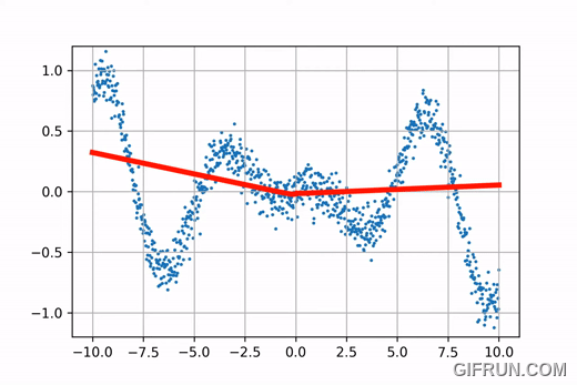
What if we have more than 4 point? For instance 10 or 20 points. We can follow the same procedure and calculate the coefficients, but observe that the curves will just behave in a crazy fashion, will have a lot of noise and will be non-smooth.

In order to solve this issue, we try to define a piecewise function, composed of functions of lower order such that the resulting piecewise function is contiuous and differentible in the given domain. For simplicity, let’s take the order to be 3. Assume that we need to interpolate $n$ points on a cartesian plane to form a curve. Consider the first two points. Assume the slope of tangents at these 2 points and then fit a cubic polynomial between these points. Repeat this for all consecutive pairs of points, hence obtaining $(n-1)$ cubic polynomials. Observe that each control point (except the endpoints) is common in 2 curves, and a slope of tangent is defined for that point for both the curves. If the slope defined is unequal, the resulting piecewise function will no longer be differtiable. Such a condition is called a knot; and in order to prevent this, we keep the left hand derivative equal to the right hand derivative for each point. In this way, we are able to define out function using $3n-2$ parameters: $n$ points, with each point having 2 values and $n-2$ values of slopes.

This gives rise to a smooth enough curve which does not go crazy like those higher degree curves. Note that we ensure that the function is continuous and differentiable at least once. This type of continuity is called the $C^1$ continuity.

In order to reduce the parameters, let’s set the slope of the tangent at the $i^{th}$ point as the slope of the line joining the $(i-1)^{th}$ and $(i+1)^{th}$ point. Such a class of splines are called Catmull-Rom Splines.

2.3.3| Pretty Natural Curves

Let’s get back to our initial condition: 3 points (2 end points and one knot point in the middle). To fit 2 cubic curves, we require 8 variables, hence 8 consistent linear equations. We get 4 equations by substituting the control points (2 points each for the 2 cubic curves). To ensure differentiability, we equate the derivatives of both curves at the knot point. Let’s also make the second derivatives equal at the knot point for ensuring that the final function is twice differentiable. We not have 6 equations. Such a spline which is continuous, has a continuous first and second derivative is called a $C^2$ spline. The fact that the spline interpolates all the control points, it is a $C^2$ interpolating spline.

Then, we make the second derivatives of end points to be 0, providing us with 8 equations and now we can sufficiently solve for the curves. This additional property makes these splines fall under the class of “Natural Cubic Splines”.

Go ahead and play with these curves using the interactive plots presented below!

If you fiddle around with the control points of the Catmull-Rom Splines and Natural Cubic Splines, you’ll notice that if you alter the position of a control point in C-R Spline, change is only observed in the cubic curves controlled by that control point, and the rest of the curve is almost unchanged. This property is called “Local Control”. On the other hand, this property is not observed in the Natural Cubic Splines. Go back to the interactive curves and fiddle with them a bit more to get a hang of it.

2.3.4| B-Splines

$C^2$ continuity offers greater smoothness to the curve, and local control provides the ability to change a function locally without altering the rest of the curve. This is an important feature when it comes to learning algorithms because local control provides greater retention and memory (more on that in Chapter 3, for now just assume that it is important). B-Splines are piecewise functions, wherein each piece is a Cubic Bezier Curve. A Bezier Curve defined by a parametric equation

Chapter 3| The Kolmogorov–Arnold Network

3.1| Architecture

Assume we have a task at hand that we are given data points ${x_1,x_2,….x_n,y}$ and need to find an $f(x_i)$ such that $f(x_i)\approx y$ (consider the housing price prediction problem). Now the KART states that if we can find $\Phi _q$ and $\phi _{q,p}$ from the below equation then we are done.

Now in order to find the uni-variate functions $\Phi _q$ and $\phi _{q,p}$ we just use splines, specifically the B-splines. But now we encounter a problem again, even though this can be easily implemented, this network would be too simple to learn things.What the network currently is, is just a 2 layern equivalent of a MLP. In order to make this network more complex and deeper, we need to add more “layers” ,but how do we do so?? The answer comes from looking at MLPs and KANs in parallel.

When we describe a MLP layer with n inputs $(a_1,…a_n)$ and m outputs $(b_1,…b_m)$ what we are essentially doing is multiplying input values with learned weights and adding biases(a linear transformation) and then passing these values through a non-linear function. Now we can add more of these layers on top of one another to make the network deeper. Now how do we make a KAN “deeper”? Before answering this question we will have to first define what a “layer” means for KAN.

The original paper says

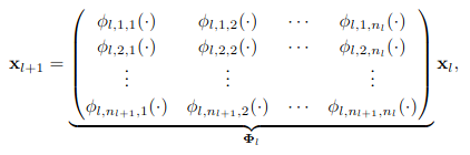
It turns out that a KAN layer with $n_in$-dimensional inputs and $n_out$-dimensional outputs can be defined as a matrix of 1D functions where the functions $\phi_{q,p}$ have trainable parameters.

Now let me explain what exactly is happening over here, say $(a_1,…a_n)$ are the n inputs and $(b_1,…b_m)$ are the m outputs then the first step is to define $m$ functions ${\phi_{1,i},\phi_{2,i},…,\phi_{m,i}}$ for each of the $i \in (1,2,…,n)$ (a total of $m * n$ functions). Now for the next step we pass through each of our input $a_i$ through the functions ${\phi_{1,i},\phi_{2,i},….\phi_{m,i}}$ defined for it to get values ${\phi _{1,i}(a_i) ,\phi _{2,i}(a_i),….\phi _{m,i}(a_i)}$ (a total of $m * n$ values). Finally to get the outputs $(b_1,…b_m)$ we calculate $b _j = \sum _{i=1}^n \phi _{j,i}(a _i)$ and voila.

Another way to interpret whats written above is by looking at the following matrix multiplication equation. I have taken this directly from the paper. Here they have taken the input dimension to be n and output dimension to be 2n+1. Now they have described the matrix to be a matrix of functions and the input and output to be column matrices. Just remember that what is going on over here is not matrix multiplication but rather the multiplication of the two elements of the matrix has been replaced by passing ones element as an argument to the function i.e. $b _{i,j} * a _{j,k} \rightarrow b(a _{j,k}) _{i,j}$

3.2| Interpretability

We have talked a lot about interpretability in this article, what it basically means is the ability to decipher how much and in what ways a given input variable affects the output(eg. how the cost relates to the no of units sold, or say how the appearance of aa shape in an immage relates to it belonging to a particular class). One of the main reasons that KANs are gaining popularity at such a pace is because of their improved interpretability. MLPs are known as black-boxes because after going through multiple transformations (multiplication by weights) and then being passed on through activation functions , tracing these transformations from the input to the output is barely doable (its like being asked to tell all the ingredients present in a dish you have never tasted in your life). The non linear activation functions are what really make MLPs very hard to interpret because they modify the input in very non interpretable way (think of how tanh and sigmoid squishify stuff). Now in KANs since we do not multiply inputs with weights and only ever pass it through activation functions, in addition to which the activation functions are also learnable splines(much more ‘readable’), they become much more interpretable by humans. We can very easily see how the input value translates to the output value as the activation functions are much easily visualized. This interpretability in KANs makes them particularly useful in scientific applications where understanding how the model arrives at its results is crucial.

3.3| Applications

Okay lets draw two parallels again, between a layer of MLP and a layer of KAN. Since both do the same thing i.e. taking n inputs and giving out m outputs, even though by using different methods. So wherever the MLP layer (a fully connected layer) is used, it can be replaced by a KAN layer, given we use the correct training methods. So yes, simple neural networks can be fully replaced by KANs very easily.

But what about other neural networks such as CNNs or Transformers. How do you find the ‘KA-equivalent’ of a Convolutional layer ? Well, Machine Learning is one of the fastest developing sectors. The paper on KANs was released on 30 Apr 2024 and not even a month and a half later on 13 Jun 2024 a paper titled Suitability of KANs for Computer Vision: A preliminary investigation was released exploring the application of KAN concepts in computer vision tasks mainly classification). They did so by defining the KAN convolution layer which does work in a similar way to a KAN layer, that is by eliminating the weights and biases and changing the activation functions to learnable splines. This paper does go out of scope for this article but the key takeaways are that KConvKANs do outperform traditional CNNs on small sized datasets such as MNIST but on slightly bigger datasets such as CIFAR-10 , the margin by which they outperform them becomes pretty minuscule.(Note-the comparisons made here are based on the number of parameters)

Integrating KANs in Large Language Models(LLMs) could provide a window into how these models process and generate language. This could lead to more interpretable and efficient LLMs. It has not been done yet, but if KANs do turn out to be better at this task than MLPs then they potentially could revamp the whole LLM scene. But one thng to keep in mind is that they are still a “work-in-progress” thing and optimization of such new techniques takes its time. There have been proposed models though such as Temporal-KANs and Temporal-Kolmogorov Arnold Transformer(TKAT) that try to mimic and replace the existing LSTMs and Transformers based on MLPs.

3.4| Advantages and drawbacks

Now even though many new things are developed in the world, but they don’t gain traction unless they are better than previously existing solutions.KANs also have to have some benefits over MLPs given their popularity. Lets take a look at some of those.

1. Interpretability - We have talked about it a lot in the previous headings so i wont repeat the same things here again
2. Efficiency- KANs are indeed a large step up from MLPs in terms of accuracy with a lower number of parameters. With a lower number of parameters KANs can produce the same or better results than MLPs. This means a smaller model with better accuracy(who doesn’t want that).
3. Complexity Handling- KANs are inherently better at handling complex data because they use sum of splines to represent these functions. They can also do so by using much less parameters in comparison to MLPs. Using sum of splines to represent a function allows KANs to capture much more detail because splines themselves can capture relations between input and output much better.

Though KANs have their benefits over MLPs, they have their drawbacks as well:

1. Training time- Some researches do suggest that KANs should converge faster but currently they do not.This is because MLPs take advantage of GPU parallelization and optimized techniques for matrix multiplications and training. Such techniques have not yet been developed for KANs and thus they are slower to train.
2. Computational Resources- KANs being new have not been optimized to make them efficient and thus they take up a lot of computation resources to train. Moreover the use of splines make them more computationally heavy than MLPs as matrix operations have been heavily optimized .

3.5| Current stage of development

Given how promising KANs are, it should not be very surprising that it has seen a plethora of developments towards it current and upcoming applications

1. KConvKAN- KConvKAN are an architecture based entirely on KAN Linear layers and KANConv layers. These, as talked about before, are currently being developed for image processing tasks using the KAN-Convolution layer based on the KAN layer and the classic convolutional layer.
2. TKAN(Temporal-KAN) - Temporal KANs were made by combining KANs and LSTMs in order to perform time series analysis. The structure of their architecture in comparison to LSTMs is quite similar but the key differenct is the use of Recurring-KAN layer. Recurring Kolmogorov-Arnold Networks (RKANs) layers integrate memory management capabilities into the network. This allows the model to better capture and retain the long-term dependencies in the input data, leading to significant improvements in the accuracy and efficiency of multi-step time series forecasting.
3. TKAT(Temporal Kolmogorov Arnold Transformer)- Why stop at RNNs and LSTMs? Researchers proposed Temporal Kolmogorov Arnold Transformer that takes its concepts from KANs and the Transformer architecture. Integration of these two provided very effective capturing of long-term and short-term memory in complex time-series data. TKAT shows a lot of promise and is a significant step forward in time-series forecasting. Who knows, maybe the future LLMs would be based on TKATs.
4. DeepOKAN- DeepOKAN is a Deep Operator network based on KAN. The key innovation here is that DeepOKAN uses Gaussian radial basis functions (RBFs) rather than the B-splines. There have already been techniques to efficiently handle RBFs, so they can be applied in the case of DeepOKANs which in turn makes them more efficient than normal KANs. They were developed to handle complex engineering scenario predictions and computational mechanics.
5. WavKAN- WavKAN is another recent development inspired by Kolmogorov-Arnold Networks (KANs). It was aimed at improving traditional KANs and addressing some of their limitations. It introduces the use of wavelet functions into the KANs. Wavelets are mathematical tools used to analyze data at different scales, capturing both high-frequency (details) and low-frequency (overall trends) information. WavKAN can reportedly achieve better accuracy and train faster compared to traditional KANs (Spline-KAN) and MLPs and they also can adapt to the specific structure of the data, leading to increased robustness.

3.6| Do It Yourself

We have talked a lot about splines and KANs and their architecture so how about getting some hands-on experience with them. Follow the given colab notebook to try KANs out and see for yourself how they fare against MLPs.

_Authors: Anirudh Singh, Himanshu Sharma