Technical Blog on Generative Adverserial Networks

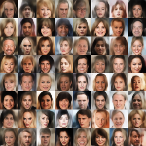
Neural networks , especially convolutional neural networks, have a lot to offer than classification tasks and its optimization. Variational autoencoders are an example of a use case of CNN lets you generate new images by learning the probability distribution of the images of the input dataset . Although they are currently inferior to the state of the art networks for similar usecase, i.e GANs , a fully probabilistic approach for Variational autoencoders make them quite interesting to explore.
Let us begin. We’ll start with a deep dive into pros and cons of autoencoders and KL divergence .
An autoencoder network is a pair of two connected networks- an encoder and a decoder. An encoder network takes in an input, and converts it into a smaller, dense representation, which the decoder network can use to convert it back to the original input. Usually , the convolutional layers of any CNN take in a large image (eg. rank 3 tensor of size 28x28x3), and convert it to a much more compact, dense representation (eg. rank 1 tensor of size 10) which is then used by the fully connected classifier network to classify the image. Similary, the encoder network takes in an input and produces a much smaller representation that contains enough information for the decoder network to process and convert it into the desired output format. Autoencoders take this idea, and slightly flip it on its head, by making the encoder generate encodings specifically useful for reconstructing its own input.
The entire network is usually trained as a whole. The loss function is usually either the mean-squared error or cross-entropy between the output and the input, known as the reconstruction loss, which penalizes the network for creating outputs different from the input.
As the encoding has far less units than the input, the encoder must choose to discard information. The encoder learns to preserve as much of the relevant information as possible and discards the irrelevant stuff. The decoder learns to take the encoding and reconstruct it into a proper image. Together, they form an autoencoder network which indeed is quite successful in reconstructing the input data .

Standard autoencoders learn to generate compact representations and reconstruct their inputs well to a good accuracy level but the input data does not cover the entire latent space (where encoded vectors lie) . Due to this discontinuous latent space, the purpose of generating new data is not served by simple autoencoders . For example, training an autoencoder on the MNIST dataset, and visualizing the encodings from a 2D latent space reveals the formation of distinct clusters. This makes sense, as distinct encodings for each image type makes it far easier for the decoder to decode them. This is fine if you’re just replicating the same images. But when you’re building a generative model, you don’t want to prepare to replicate the same image you put in. You want to randomly sample from the latent space, or generate variations on an input image, from a continuous latent space. If the space has discontinuities (eg. gaps between clusters) and you sample/generate a variation from there, the decoder will simply generate an unrealistic output, because the decoder has no idea how to deal with that region of the latent space.
Variational Autoencoders (VAEs) have one fundamentally unique property that differentiates them from autoencoders : their latent spaces are, by design, continuous, allowing easy random sampling .This property that makes them so useful and accurate for generating data
In this post we’re going to take a look at way of comparing two probability distributions called Kullback-Leibler Divergence (often shortened to just KL divergence). Very often in Probability and Statistics, we’ll replace observed data or a complex distributions with a simpler, approximating distribution. KL Divergence helps us to measure just how much information we lose when we choose an approximation.
KL Divergence has its origins in information theory. The primary goal of information theory is to measure how much information is in data. The most important metric in information theory is called Entropy, typically denoted as H. Entropy of a probability distribution is defined as following :
,where common values of b are 2 or e and P(X) denotes the Probability mass function .
Kullback-Leibler Divergence is just a slight modification of our formula for entropy. Rather than just having our probability distribution P ,we measure the difference of the log values of the approximating probability distribution Q


Relating this with entropy,
where H(P,Q) is the cross entropy of P and Q.
We can observe here that by minimizing the KL divergence of two probability distributions , we can make our approximating distribution more closer to the actual probability distribution and this optimization is tractable .Combining KL divergence with neural networks allows us to learn very complex approximating distribution for our data and this approach is used Variational Autoencoders .
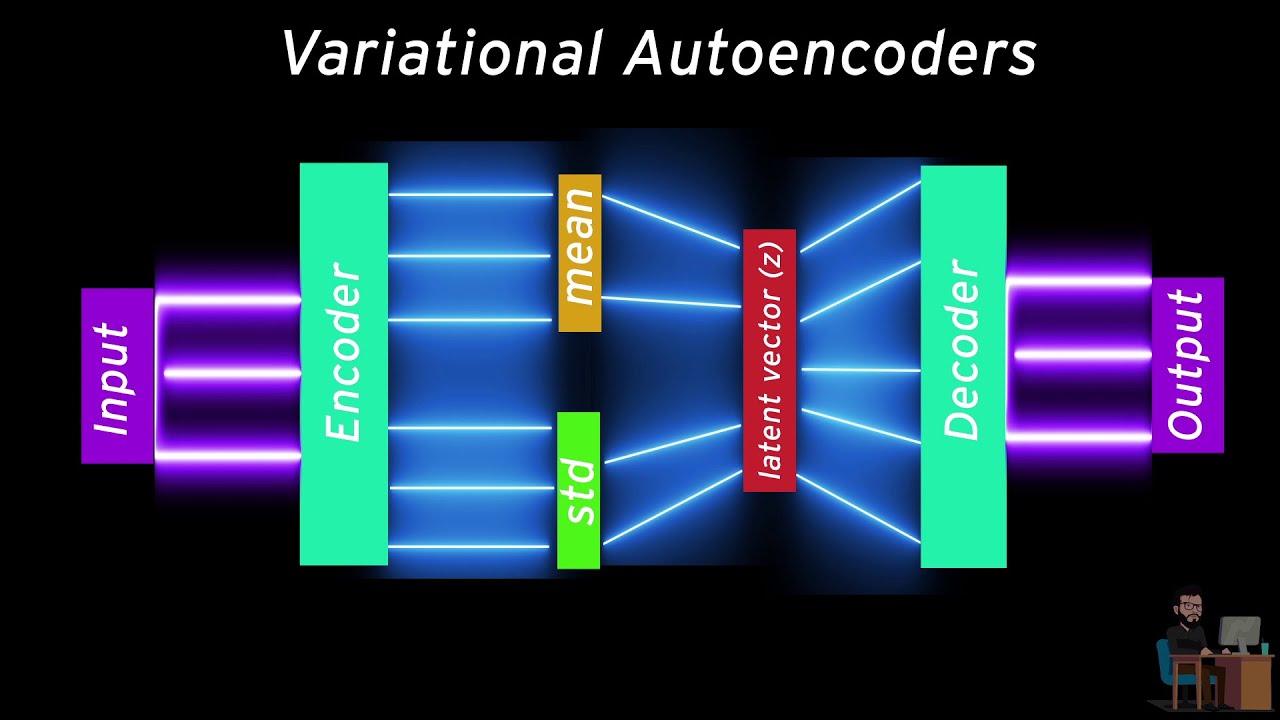
The unique property in VAEs which makes them so useful in maing generative models is that their latent space is continuous which allows random sampling .This happens because its encoder does not output an encoding vector of size n, rather, outputs two vectors of size n: a vector of means, μ, and another vector of standard deviations, σ . μ and σ now become the parameters for a vector of size n containing random values having mean and standard deviation as μ and σ respectively . This will result in random generation of data having mean and standard deviation close to the input data.
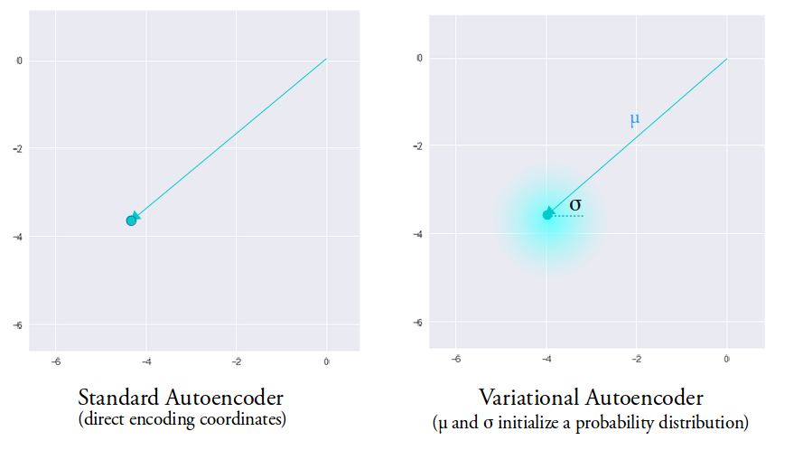
Hence,the mean vector controls where the encoding of an input should be centered around, while the standard deviation controls the area, how much from the mean the encoding can vary. As encodings are generated at random from anywhere inside the shaded portion, the decoder learns all the nearby points that refer to sample of that class . This allows the decoder to not just decode specific encodings in the latent space but also the ones which vary thus making the latent space continuous .
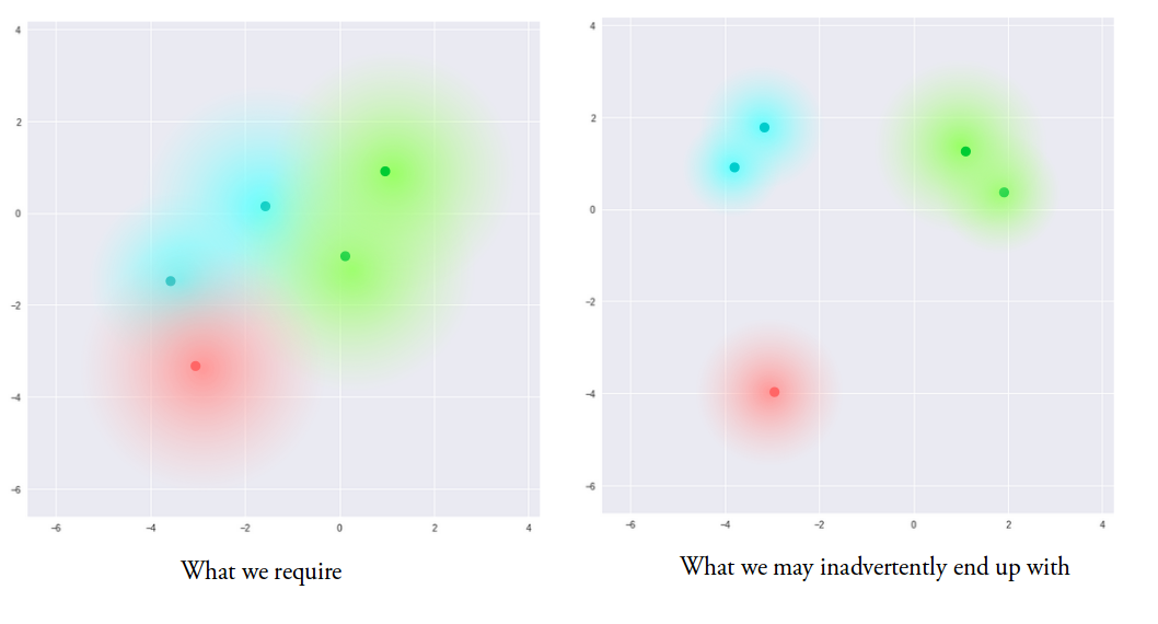
We want our encodings to be as close as possible while still being distinct to make smooth interpolation, but sometimes we might end up making our latent space similar to the right picture shown above as there are no limits on what values vectors μ and σ can take on, so to avoid this , we introduce KL divergence in the loss function .
The following image shows the calculation of the log of the data likelihood
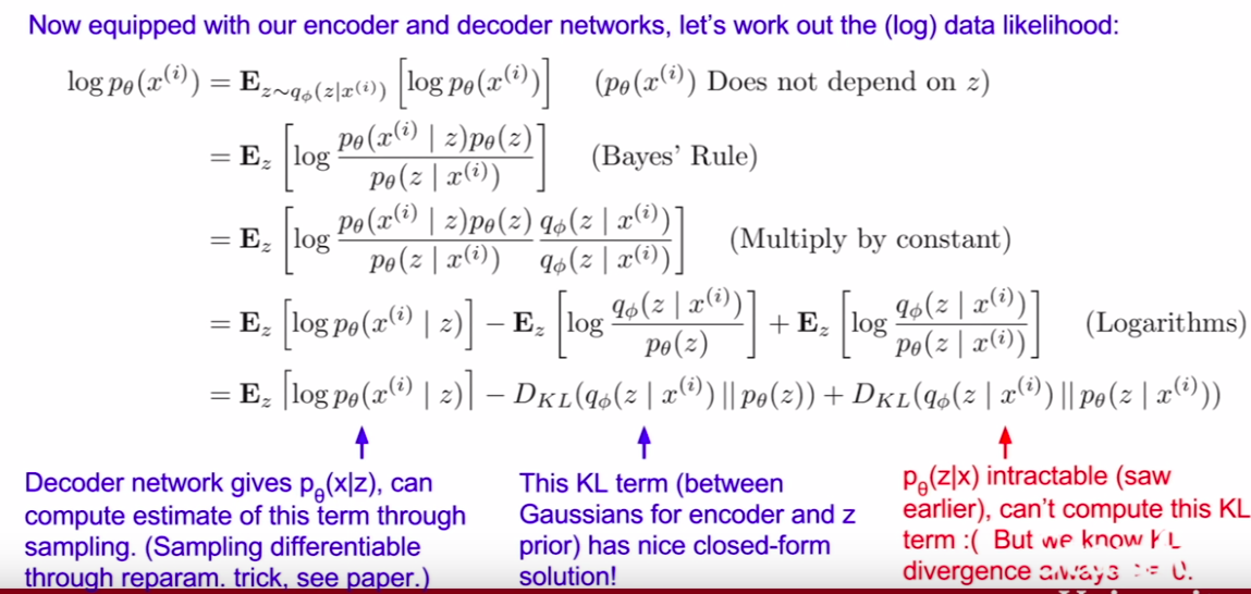
| Although the third term in intractable, by Gibbs inequality , we know that KL divergence of two distributions is always non-negative . Hence, the first two terms can be a tractable lower bound to the log data likelihood which we can easily differentiate (P(X | Z) is mostly a simple distribution like Guassian and KL term is also differntiable ) and hence optimize .The combination of first two terms is also known as Variational Lower Bound (“ELBO”) . The first term here is responsible for reconstructing the original input data and the second term is responsible for making approximate distribution close to input distribution . |
So I guess this is enough for a start. There is much to learn, but perhaps that would be covered in another article. I present to you a few useful links: